jueves, 26 de octubre de 2017

Curso de introducción a python aplicado a la adquisición de datos de audio

Curso de introducción a python aplicado a la adquisición de datos de audio


Grupo de Estudio en Modelamiento Matemático 


Computo Científico

Alexander Arias
Septiembre de 2017

Sesión 1. Introducción a Python y PyCharm
https://cloud.mail.ru/public/Jty6/LJ9bkFcFX

Sesión 2. Operadores Básicos en Consola y primera aplicación con entrada de datos en PyCharm
https://cloud.mail.ru/public/aJBq/BABnXE7dU

Sesión 3. Listas, Strings y Operaciones básicas con Strings
https://cloud.mail.ru/public/LkX5/jhbzEzhpo

Sesión 4. Diccionarios, Condicionales, Excepciones y Loops
https://cloud.mail.ru/public/92UX/Z8SWPHmRF

Octubre 2017

Sesión 5. Funciones, Módulos y paquetes. Adquisición de datos de un sensor Ultrasonico por medio del puerto serial
https://cloud.mail.ru/public/DLXS/HSw8kSyRq

 Sesión 6. Objetos e Interfaces Gráficas GUIs
https://cloud.mail.ru/public/3HX4/BoVuG1cVB

jueves, 19 de octubre de 2017

Solucion Problema Excel Microsoft no puede abrir o guardar mas documentos porque el espacio en disco o la memoria son insuficientes

Solución

Solucion Problema Excel Microsoft no puede abrir o guardar mas documentos porque el espacio en disco o la memoria son insuficientes


La forma más sencilla y rápida de solucionar este problema, una vez se presente por causa de cambio de versión de Office, es realizar lo siguiente:

1. Cerrar completamente el archivo.

2. Hacer clic derecho sobre él y seleccionar Propiedades.

En la ventana de Propiedades verán en la parte inferior un botón adicional que dice: Desbloquear:
Imagen
3. Hacer clic en el botón Desbloquear, Aplicar y Aceptar.

Una vez hecho esto, el archivo se podrá abrir sin ningún tipo de problemas nuevamente y los ADS quedarán borrados.

Esto lo encontre en el hilo
 respondió el 

sábado, 14 de octubre de 2017

Objetos en Python Tortugas que se mueven y dibujan en línea Online Run

Objetos en Python Tortugas que se mueven y dibujan en línea Online Run
https://hourofpython.com/una-introduccion-visual-a-python/index.html


Python Recursion Drawing Fractals

Python Recursion Drawing Fractals


http://openbookproject.net/thinkcs/python/english3e/recursion.html

 How to Think Like a Computer Scientist: Learning with Python 3

18. Recursion

Recursion means “defining something in terms of itself” usually at some smaller scale, perhaps multiple times, to achieve your objective. For example, we might say “A human being is someone whose mother is a human being”, or “a directory is a structure that holds files and (smaller) directories”, or “a family tree starts with a couple who have children, each with their own family sub-trees”.
Programming languages generally support recursion, which means that, in order to solve a problem, functions can call themselves to solve smaller subproblems.

18.1. Drawing Fractals

For our purposes, a fractal is a drawing which also has self-similar structure, where it can be defined in terms of itself.
Let us start by looking at the famous Koch fractal. An order 0 Koch fractal is simply a straight line of a given size.
_images/koch_0.png 
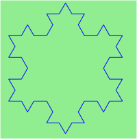
An order 1 Koch fractal is obtained like this: instead of drawing just one line, draw instead four smaller segments, in the pattern shown here:
_images/koch_1.png Now what would happen if we repeated this Koch pattern again on each of the order 1 segments? We’d get this order 2 Koch fractal:
_images/koch_2.png 
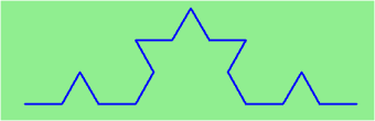
Repeating our pattern again gets us an order 3 Koch fractal:
_images/koch_3.png 
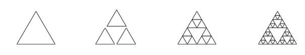
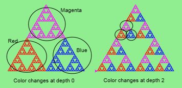
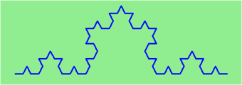
Now let us think about it the other way around. To draw a Koch fractal of order 3, we can simply draw four order 2 Koch fractals. But each of these in turn needs four order 1 Koch fractals, and each of those in turn needs four order 0 fractals. Ultimately, the only drawing that will take place is 
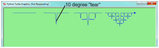
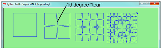
at order 0. This is very simple to code up in Python:
 1
 2
 3
 4
 5
 6
 7
 8
 9
10
11
12
13
14
15
16
def koch(t, order, size):
    """
       Make turtle t draw a Koch fractal of 'order' and 'size'.
       Leave the turtle facing the same direction.
    """

    if order == 0:          # The base case is just a straight line
        t.forward(size)
    else:
        koch(t, order-1, size/3)   # Go 1/3 of the way
        t.left(60)
        koch(t, order-1, size/3)
        t.right(120)
        koch(t, order-1, size/3)
        t.left(60)
        koch(t, order-1, size/3)
The key thing that is new here is that if order is not zero, koch calls itself recursively to get its job done.
Let’s make a simple observation and tighten up this code. Remember that turning right by 120 is the same as turning left by -120. So with a bit of clever rearrangement, we can use a loop instead of lines 10-16:
1
2
3
4
5
6
7
def koch(t, order, size):
    if order == 0:
        t.forward(size)
    else:
        for angle in [60, -120, 60, 0]:
           koch(t, order-1, size/3)
           t.left(angle)
The final turn is 0 degrees — so it has no effect. But it has allowed us to find a pattern and reduce seven lines of code to three, which will make things easier for our next observations.
Recursion, the high-level view
One way to think about this is to convince yourself that the function works correctly when you call it for an order 0 fractal. Then do a mental leap of faith, saying “the fairy godmother (or Python, if you can think of Python as your fairy godmother) knows how to handle the recursive level 0 calls for me on lines 11, 13, 15, and 17, so I don’t need to think about that detail!” All I need to focus on is how to draw an order 1 fractal if I can assume the order 0 one is already working.
You’re practicing mental abstraction — ignoring the subproblem while you solve the big problem.
If this mode of thinking works (and you should practice it!), then take it to the next level. Aha! now can I see that it will work when called for order 2 under the assumption that it is already working for level 1.
And, in general, if I can assume the order n-1 case works, can I just solve the level n problem?
Students of mathematics who have played with proofs of induction should see some very strong similarities here.
Recursion, the low-level operational view
Another way of trying to understand recursion is to get rid of it! If we had separate functions to draw a level 3 fractal, a level 2 fractal, a level 1 fractal and a level 0 fractal, we could simplify the above code, quite mechanically, to a situation where there was no longer any recursion, like this:
 1
 2
 3
 4
 5
 6
 7
 8
 9
10
11
12
13
14
15
16
17
def koch_0(t, size):
    t.forward(size)

def koch_1(t, size):
    for angle in [60, -120, 60, 0]:
       koch_0(t, size/3)
       t.left(angle)

def koch_2(t, size):
    for angle in [60, -120, 60, 0]:
       koch_1(t, size/3)
       t.left(angle)

def koch_3(t, size):
    for angle in [60, -120, 60, 0]:
       koch_2(t, size/3)
       t.left(angle)
This trick of “unrolling” the recursion gives us an operational view of what happens. You can trace the program into koch_3, and from there, into koch_2, and then into koch_1, etc., all the way down the different layers of the recursion.
This might be a useful hint to build your understanding. The mental goal is, however, to be able to do the abstraction!

18.2. Recursive data structures

All of the Python data types we have seen can be grouped inside lists and tuples in a variety of ways. Lists and tuples can also be nested, providing many possibilities for organizing data. The organization of data for the purpose of making it easier to use is called a data structure.
It’s election time and we are helping to compute the votes as they come in. Votes arriving from individual wards, precincts, municipalities, counties, and states are sometimes reported as a sum total of votes and sometimes as a list of subtotals of votes. After considering how best to store the tallies, we decide to use a nested number list, which we define as follows:
A nested number list is a list whose elements are either:
  1. numbers
  2. nested number lists
Notice that the term, nested number list is used in its own definition. Recursive definitions like this are quite common in mathematics and computer science. They provide a concise and powerful way to describe recursive data structures that are partially composed of smaller and simpler instances of themselves. The definition is not circular, since at some point we will reach a list that does not have any lists as elements.
Now suppose our job is to write a function that will sum all of the values in a nested number list. Python has a built-in function which finds the sum of a sequence of numbers:
>>> sum([1, 2, 8])
11
For our nested number list, however, sum will not work:
>>> sum([1, 2, [11, 13], 8])
Traceback (most recent call last):
  File "<interactive input>", line 1, in <module>
TypeError: unsupported operand type(s) for +: 'int' and 'list'
>>>
The problem is that the third element of this list, [11, 13], is itself a list, so it cannot just be added to 1, 2, and 8.

18.3. Processing recursive number lists

To sum all the numbers in our recursive nested number list we need to traverse the list, visiting each of the elements within its nested structure, adding any numeric elements to our sum, and recursively repeating the summing process with any elements which are themselves sub-lists.
Thanks to recursion, the Python code needed to sum the values of a nested number list is surprisingly short:
1
2
3
4
5
6
7
8
def r_sum(nested_num_list):
    tot = 0
    for element in nested_num_list:
        if type(element) == type([]):
            tot += r_sum(element)
        else:
            tot += element
    return tot
The body of r_sum consists mainly of a for loop that traverses nested_num_list. If element is a numerical value (the else branch), it is simply added to tot. If element is a list, then r_sum is called again, with the element as an argument. The statement inside the function definition in which the function calls itself is known as the recursive call.
The example above has a base case (on line 13) which does not lead to a recursive call: the case where the element is not a (sub-) list. Without a base case, you’ll have infinite recursion, and your program will not work.
Recursion is truly one of the most beautiful and elegant tools in computer science.
A slightly more complicated problem is finding the largest value in our nested number list:
 1
 2
 3
 4
 5
 6
 7
 8
 9
10
11
12
13
14
15
16
17
18
19
20
21
22
23
24
def r_max(nxs):
    """
      Find the maximum in a recursive structure of lists
      within other lists.
      Precondition: No lists or sublists are empty.
    """
    largest = None
    first_time = True
    for e in nxs:
        if type(e) == type([]):
            val = r_max(e)
        else:
            val = e

        if first_time or val > largest:
            largest = val
            first_time = False

    return largest

test(r_max([2, 9, [1, 13], 8, 6]) == 13)
test(r_max([2, [[100, 7], 90], [1, 13], 8, 6]) == 100)
test(r_max([[[13, 7], 90], 2, [1, 100], 8, 6]) == 100)
test(r_max(["joe", ["sam", "ben"]]) == "sam")
Tests are included to provide examples of r_max at work.
The added twist to this problem is finding a value for initializing largest. We can’t just use nxs[0], since that could be either a element or a list. To solve this problem (at every recursive call) we initialize a Boolean flag (at line 8). When we’ve found the value of interest, (at line 15) we check to see whether this is the initializing (first) value for largest, or a value that could potentially change largest.
Again here we have a base case at line 13. If we don’t supply a base case, Python stops after reaching a maximum recursion depth and returns a runtime error. See how this happens, by running this little script which we will call infinite_recursion.py:
1
2
3
4
5
def recursion_depth(number):
    print("{0}, ".format(number), end="")
    recursion_depth(number + 1)

recursion_depth(0)
After watching the messages flash by, you will be presented with the end of a long traceback that ends with a message like the following:
RuntimeError: maximum recursion depth exceeded ...
We would certainly never want something like this to happen to a user of one of our programs, so in the next chapter we’ll see how errors, any kinds of errors, are handled in Python.

18.4. Case study: Fibonacci numbers

The famous Fibonacci sequence 0, 1, 1, 2, 3, 5, 8, 13, 21, 34, 55, 89, 134, ... was devised by Fibonacci (1170-1250), who used this to model the breeding of (pairs) of rabbits. If, in generation 7 you had 21 pairs in total, of which 13 were adults, then next generation the adults will all have bred new children, and the previous children will have grown up to become adults. So in generation 8 you’ll have 13+21=34, of which 21 are adults.
This model to explain rabbit breeding made the simplifying assumption that rabbits never died. Scientists often make (unrealistic) simplifying assumptions and restrictions to make some headway with the problem.
If we number the terms of the sequence from 0, we can describe each term recursively as the sum of the previous two terms:
fib(0) = 0
fib(1) = 1
fib(n) = fib(n-1) + fib(n-2)  for n >= 2
This translates very directly into some Python:
1
2
3
4
5
def fib(n):
    if n <= 1:
        return n
    t = fib(n-1) + fib(n-2)
    return t
This is a particularly inefficient algorithm, and we’ll show one way of fixing it when we learn about dictionaries:
1
2
3
4
5
6
7
import time
t0 = time.clock()
n = 35
result = fib(n)
t1 = time.clock()

print("fib({0}) = {1}, ({2:.2f} secs)".format(n, result, t1-t0))
We get the correct result, but an exploding amount of work!
fib(35) = 9227465, (10.54 secs)

18.5. Example with recursive directories and files

The following program lists the contents of a directory and all its subdirectories.
 1
 2
 3
 4
 5
 6
 7
 8
 9
10
11
12
13
14
15
16
17
18
19
20
21
22
23
import os

def get_dirlist(path):
    """
      Return a sorted list of all entries in path.
      This returns just the names, not the full path to the names.
    """
    dirlist = os.listdir(path)
    dirlist.sort()
    return dirlist

def print_files(path, prefix = ""):
    """ Print recursive listing of contents of path """
    if prefix == "":  # Detect outermost call, print a heading
        print("Folder listing for", path)
        prefix = "| "

    dirlist = get_dirlist(path)
    for f in dirlist:
        print(prefix+f)                    # Print the line
        fullname = os.path.join(path, f)   # Turn name into full pathname
        if os.path.isdir(fullname):        # If a directory, recurse.
            print_files(fullname, prefix + "| ")
Calling the function print_files with some folder name will produce output similar to this:
Folder listing for c:\python31\Lib\site-packages\pygame\examples
| __init__.py
| aacircle.py
| aliens.py
| arraydemo.py
| blend_fill.py
| blit_blends.py
| camera.py
| chimp.py
| cursors.py
| data
| | alien1.png
| | alien2.png
| | alien3.png
...

18.6. An animated fractal, using PyGame

Here we have a tree fractal pattern of order 8. We’ve labelled some of the edges, showing the depth of the recursion at which each edge was drawn.
_images/recursivetree1.png 
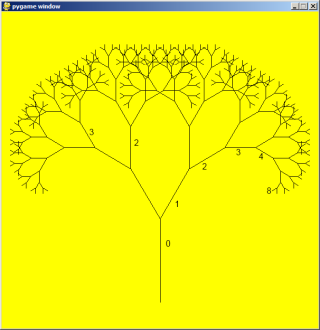
In the tree above, the angle of deviation from the trunk is 30 degrees. Varying that angle gives other interesting shapes, for example, with the angle at 90 degrees we get this:
_images/recursivetree2.png 
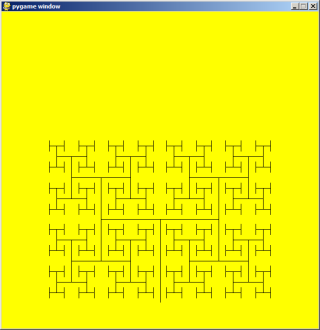
An interesting animation occurs if we generate and draw trees very rapidly, each time varying the angle a little. Although the Turtle module can draw trees like this quite elegantly, we could struggle for good frame rates. So we’ll use PyGame instead, with a few embellishments and observations. (Once again, we suggest you cut and paste this code into your Python environment.)
 1
 2
 3
 4
 5
 6
 7
 8
 9
10
11
12
13
14
15
16
17
18
19
20
21
22
23
24
25
26
27
28
29
30
31
32
33
34
35
36
37
38
39
40
41
42
43
44
45
46
47
48
49
50
51
52
53
54
55
56
57
58
59
60
import pygame, math
pygame.init()           # prepare the pygame module for use

# Create a new surface and window.
surface_size = 1024
main_surface = pygame.display.set_mode((surface_size,surface_size))
my_clock = pygame.time.Clock()


def draw_tree(order, theta, sz, posn, heading, color=(0,0,0), depth=0):

   trunk_ratio = 0.29       # How big is the trunk relative to whole tree?
   trunk = sz * trunk_ratio # length of trunk
   delta_x = trunk * math.cos(heading)
   delta_y = trunk * math.sin(heading)
   (u, v) = posn
   newpos = (u + delta_x, v + delta_y)
   pygame.draw.line(main_surface, color, posn, newpos)

   if order > 0:   # Draw another layer of subtrees

      # These next six lines are a simple hack to make the two major halves
      # of the recursion different colors. Fiddle here to change colors
      # at other depths, or when depth is even, or odd, etc.
      if depth == 0:
          color1 = (255, 0, 0)
          color2 = (0, 0, 255)
      else:
          color1 = color
          color2 = color

      # make the recursive calls to draw the two subtrees
      newsz = sz*(1 - trunk_ratio)
      draw_tree(order-1, theta, newsz, newpos, heading-theta, color1, depth+1)
      draw_tree(order-1, theta, newsz, newpos, heading+theta, color2, depth+1)


def gameloop():

    theta = 0
    while True:

        # Handle evente from keyboard, mouse, etc.
        ev = pygame.event.poll()
        if ev.type == pygame.QUIT:
            break;

        # Updates - change the angle
        theta += 0.01

        # Draw everything
        main_surface.fill((255, 255, 0))
        draw_tree(9, theta, surface_size*0.9, (surface_size//2, surface_size-50), -math.pi/2)

        pygame.display.flip()
        my_clock.tick(120)


gameloop()
pygame.quit()
  • The math library works with angles in radians rather than degrees.
  • Lines 14 and 15 uses some high school trigonmetry. From the length of the desired line (trunk), and its desired angle, cos and sin help us to calculate the x and y distances we need to move.
  • Lines 22-30 are unnecessary, except if we want a colorful tree.
  • In the main game loop at line 49 we change the angle on every frame, and redraw the new tree.
  • Line 18 shows that PyGame can also draw lines, and plenty more. Check out the documentation. For example, drawing a small circle at each branch point of the tree can be accomplished by adding this line directly below line 18:
    1
    pygame.draw.circle(main_surface, color, (int(posn[0]), int(posn[1])), 3)
    
Another interesting effect — instructive too, if you wish to reinforce the idea of different instances of the function being called at different depths of recursion — is to create a list of colors, and let each recursive depth use a different color for drawing. (Use the depth of the recursion to index the list of colors.)

18.7. Glossary

base case
A branch of the conditional statement in a recursive function that does not give rise to further recursive calls.
infinite recursion
A function that calls itself recursively without ever reaching any base case. Eventually, infinite recursion causes a runtime error.
recursion
The process of calling a function that is already executing.
recursive call
The statement that calls an already executing function. Recursion can also be indirect — function f can call g which calls h, and h could make a call back to f.
recursive definition
A definition which defines something in terms of itself. To be useful it must include base cases which are not recursive. In this way it differs from a circular definition. Recursive definitions often provide an elegant way to express complex data structures, like a directory that can contain other directories, or a menu that can contain other menus.

18.8. Exercises

  1. Modify the Koch fractal program so that it draws a Koch snowflake, like this:
    _images/koch_snowflake.png

    1. Draw a Cesaro torn line fractal, of the order given by the user. We show four different lines of orders 0,1,2,3. In this example, the angle of the tear is 10 degrees.
      _images/cesaro_torn_line.png
    2. Four lines make a square. Use the code in part a) to draw cesaro squares. Varying the angle gives interesting effects — experiment a bit, or perhaps let the user input the angle of the tear.
      _images/cesaro_torn_square.png
    1. (For the mathematically inclined). In the squares shown here, the higher-order drawings become a little larger. (Look at the bottom lines of each square - they’re not aligned.) This is because we just halved the drawn part of the line for each recursive subproblem. So we’ve “grown” the overall square by the width of the tear(s). Can you solve the geometry problem so that the total size of the subproblem case (including the tear) remains exactly the same size as the original?

  2. A Sierpinski triangle of order 0 is an equilateral triangle. An order 1 triangle can be drawn by drawing 3 smaller triangles (shown slightly disconnected here, just to help our understanding). Higher order 2 and 3 triangles are also shown. Draw Sierpinski triangles of any order input by the user.
    _images/sierpinski.png
  3. Adapt the above program to change the color of its three sub-triangles at some depth of recursion. The illustration below shows two cases: on the left, the color is changed at depth 0 (the outmost level of recursion), on the right, at depth 2. If the user supplies a negative depth, the color never changes. (Hint: add a new optional parameter colorChangeDepth (which defaults to -1), and make this one smaller on each recursive subcall. Then, in the section of code before you recurse, test whether the parameter is zero, and change color.)
    _images/sierpinski_color.png
  4. Write a function, recursive_min, that returns the smallest value in a nested number list. Assume there are no empty lists or sublists:
    test(recursive_min([2, 9, [1, 13], 8, 6]) == 1)
    test(recursive_min([2, [[100, 1], 90], [10, 13], 8, 6]) == 1)
    test(recursive_min([2, [[13, -7], 90], [1, 100], 8, 6]) == -7)
    test(recursive_min([[[-13, 7], 90], 2, [1, 100], 8, 6]) == -13)
    
  5. Write a function count that returns the number of occurrences of target in a nested list:
    test(count(2, []), 0)
    test(count(2, [2, 9, [2, 1, 13, 2], 8, [2, 6]]) == 4)
    test(count(7, [[9, [7, 1, 13, 2], 8], [7, 6]]) == 2)
    test(count(15, [[9, [7, 1, 13, 2], 8], [2, 6]]) == 0)
    test(count(5, [[5, [5, [1, 5], 5], 5], [5, 6]]) == 6)
    test(count("a",
         [["this",["a",["thing","a"],"a"],"is"], ["a","easy"]]) == 4)
    
  6. Write a function flatten that returns a simple list containing all the values in a nested list:
    test(flatten([2,9,[2,1,13,2],8,[2,6]]) == [2,9,2,1,13,2,8,2,6])
    test(flatten([[9,[7,1,13,2],8],[7,6]]) == [9,7,1,13,2,8,7,6])
    test(flatten([[9,[7,1,13,2],8],[2,6]]) == [9,7,1,13,2,8,2,6])
    test(flatten([["this",["a",["thing"],"a"],"is"],["a","easy"]]) ==
                  ["this","a","thing","a","is","a","easy"])
    test(flatten([]) == [])
    
  7. Rewrite the fibonacci algorithm without using recursion. Can you find bigger terms of the sequence? Can you find fib(200)?
  8. Use help to find out what sys.getrecursionlimit() and sys.setrecursionlimit(n) do. Create several experiments similar to what was done in infinite_recursion.py to test your understanding of how these module functions work.
  9. Write a program that walks a directory structure (as in the last section of this chapter), but instead of printing filenames, it returns a list of all the full paths of files in the directory or the subdirectories. (Don’t include directories in this list — just files.) For example, the output list might have elements like this:
    ["C:\Python31\Lib\site-packages\pygame\docs\ref\mask.html",
     "C:\Python31\Lib\site-packages\pygame\docs\ref\midi.html",
     ...
     "C:\Python31\Lib\site-packages\pygame\examples\aliens.py",
     ...
     "C:\Python31\Lib\site-packages\pygame\examples\data\boom.wav",
     ... ]
  10. Write a program named litter.py that creates an empty file named trash.txt in each subdirectory of a directory tree given the root of the tree as an argument (or the current directory as a default). Now write a program named cleanup.py that removes all these files.
    Hint #1: Use the program from the example in the last section of this chapter as a basis for these two recursive programs. Because you’re going to destroy files on your disks, you better get this right, or you risk losing files you care about. So excellent advice is that initially you should fake the deletion of the files — just print the full path names of each file that you intend to delete. Once you’re happy that your logic is correct, and you can see that you’re not deleting the wrong things, you can replace the print statement with the real thing.
    Hint #2: Look in the os module for a function that removes files.

Python online "run" Recursion Fractals and Visualization trees


Python Recursion Fractals and Visualization trees
http://interactivepython.org/runestone/static/pythonds/Recursion/pythondsintro-VisualizingRecursion.html


4.7. Introduction: Visualizing Recursion

In the previous section we looked at some problems that were easy to solve using recursion; however, it can still be difficult to find a mental model or a way of visualizing what is happening in a recursive function. This can make recursion difficult for people to grasp. In this section we will look at a couple of examples of using recursion to draw some interesting pictures. As you watch these pictures take shape you will get some new insight into the recursive process that may be helpful in cementing your understanding of recursion.
The tool we will use for our illustrations is Python’s turtle graphics module called turtle. The turtle module is standard with all versions of Python and is very easy to use. The metaphor is quite simple. You can create a turtle and the turtle can move forward, backward, turn left, turn right, etc. The turtle can have its tail up or down. When the turtle’s tail is down and the turtle moves it draws a line as it moves. To increase the artistic value of the turtle you can change the width of the tail as well as the color of the ink the tail is dipped in.
Here is a simple example to illustrate some turtle graphics basics. We will use the turtle module to draw a spiral recursively. ActiveCode 1 shows how it is done. After importing the turtle module we create a turtle. When the turtle is created it also creates a window for itself to draw in. Next we define the drawSpiral function. The base case for this simple function is when the length of the line we want to draw, as given by the len parameter, is reduced to zero or less. If the length of the line is longer than zero we instruct the turtle to go forward by len units and then turn right 90 degrees. The recursive step is when we call drawSpiral again with a reduced length. At the end of ActiveCode 1 you will notice that we call the function myWin.exitonclick(), this is a handy little method of the window that puts the turtle into a wait mode until you click inside the window, after which the program cleans up and exits.
1
import turtle
2
3
myTurtle = turtle.Turtle()
4
myWin = turtle.Screen()
5
6
def drawSpiral(myTurtle, lineLen):
7
    if lineLen > 0:
8
        myTurtle.forward(lineLen)
9
        myTurtle.right(90)
10
        drawSpiral(myTurtle,lineLen-5)
11
12
drawSpiral(myTurtle,100)
13
myWin.exitonclick()
14
Drawing a Recursive Spriral using turtle (lst_turt1)
That is really about all the turtle graphics you need to know in order to make some pretty impressive drawings. For our next program we are going to draw a fractal tree. Fractals come from a branch of mathematics, and have much in common with recursion. The definition of a fractal is that when you look at it the fractal has the same basic shape no matter how much you magnify it. Some examples from nature are the coastlines of continents, snowflakes, mountains, and even trees or shrubs. The fractal nature of many of these natural phenomenon makes it possible for programmers to generate very realistic looking scenery for computer generated movies. In our next example we will generate a fractal tree.
To understand how this is going to work it is helpful to think of how we might describe a tree using a fractal vocabulary. Remember that we said above that a fractal is something that looks the same at all different levels of magnification. If we translate this to trees and shrubs we might say that even a small twig has the same shape and characteristics as a whole tree. Using this idea we could say that a tree is a trunk, with a smaller tree going off to the right and another smaller tree going off to the left. If you think of this definition recursively it means that we will apply the recursive definition of a tree to both of the smaller left and right trees.
Let’s translate this idea to some Python code. Listing 1 shows how we can use our turtle to generate a fractal tree. Let’s look at the code a bit more closely. You will see that on lines 5 and 7 we are making a recursive call. On line 5 we make the recursive call right after the turtle turns to the right by 20 degrees; this is the right tree mentioned above. Then in line 7 the turtle makes another recursive call, but this time after turning left by 40 degrees. The reason the turtle must turn left by 40 degrees is that it needs to undo the original 20 degree turn to the right and then do an additional 20 degree turn to the left in order to draw the left tree. Also notice that each time we make a recursive call to tree we subtract some amount from the branchLen parameter; this is to make sure that the recursive trees get smaller and smaller. You should also recognize the initial if statement on line 2 as a check for the base case of branchLen getting too small.
Listing 1
1
2
3
4
5
6
7
8
9
def tree(branchLen,t):
    if branchLen > 5:
        t.forward(branchLen)
        t.right(20)
        tree(branchLen-15,t)
        t.left(40)
        tree(branchLen-10,t)
        t.right(20)
        t.backward(branchLen)
The complete program for this tree example is shown in ActiveCode 2. Before you run the code think about how you expect to see the tree take shape. Look at the recursive calls and think about how this tree will unfold. Will it be drawn symmetrically with the right and left halves of the tree taking shape simultaneously? Will it be drawn right side first then left side?
1
import turtle
2
3
def tree(branchLen,t):
4
    if branchLen > 5:
5
        t.forward(branchLen)
6
        t.right(20)
7
        tree(branchLen-15,t)
8
        t.left(40)
9
        tree(branchLen-15,t)
10
        t.right(20)
11
        t.backward(branchLen)
12
13
def main():
14
    t = turtle.Turtle()
15
    myWin = turtle.Screen()
16
    t.left(90)
17
    t.up()
18
    t.backward(100)
19
    t.down()
20
    t.color("green")
21
    tree(75,t)
22
    myWin.exitonclick()
23
24
main()
25
Recursively Drawing a Tree (lst_complete_tree)
Notice how each branch point on the tree corresponds to a recursive call, and notice how the tree is drawn to the right all the way down to its shortest twig. You can see this in Figure 1. Now, notice how the program works its way back up the trunk until the entire right side of the tree is drawn. You can see the right half of the tree in Figure 2. Then the left side of the tree is drawn, but not by going as far out to the left as possible. Rather, once again the entire right side of the left tree is drawn until we finally make our way out to the smallest twig on the left.
../_images/tree1.png
../_images/tree2.png
This simple tree program is just a starting point for you, and you will notice that the tree does not look particularly realistic because nature is just not as symmetric as a computer program. The exercises at the end of the chapter will give you some ideas for how to explore some interesting options to make your tree look more realistic.
Self Check
Modify the recursive tree program using one or all of the following ideas:
  • Modify the thickness of the branches so that as the branchLen gets smaller, the line gets thinner.
  • Modify the color of the branches so that as the branchLen gets very short it is colored like a leaf.
  • Modify the angle used in turning the turtle so that at each branch point the angle is selected at random in some range. For example choose the angle between 15 and 45 degrees. Play around to see what looks good.
  • Modify the branchLen recursively so that instead of always subtracting the same amount you subtract a random amount in some range.