http://www.youtube.com/watch?v=_G6ewcEMefw
Galaconcert on International Folklore Festival Prague - The Heart of
Nations, "Theatre Na Vinohradech", 30.5. 2010, the Ensemble "Africa
Ngoma"
sábado, 23 de noviembre de 2013

La vida tiene un ritmo, está en constante movimiento. Muy Buen Video del Ritmo Africano
FOLI (there is no movement without rhythm) original version by Thomas Roebers and Floris Leeuwenberg
http://www.youtube.com/watch?v=lVPLIuBy9CY
Dedicated to the people of Baro. Please share.
Life has a rhythm, it's constantly moving.
The word for rhythm ( used by the Malinke tribes ) is FOLI.
It is a word that encompasses so much more than drumming, dancing or sound.
It's found in every part of daily life.
In this film you not only hear and feel rhythm but you see it.
It's an extraordinary blend of image and sound that
feeds the senses and reminds us all
how essential it is.
La vida tiene un ritmo, está en constante movimiento. La palabra para el ritmo (de las tribus Malinké) es Foli. Es una palabra que abarca mucho más que tocar el tambor, el baile o el sonido. Se encuentra en cada parte de la vida cotidiana. En esta película no sólo escucha y siente el ritmo, también lo vé. Es una extraordinaria mezcla de imagen y sonido que alimenta los sentidos y nos recuerda a todos lo esencial que es.
La vie a un rythme, est en mouvement constant. Le mot pour le rythme (des tribus malinké) est Foli. C'est un mot qui englobe beaucoup plus de tambours, la danse ou le son. Il se trouve dans chaque partie de la vie quotidienne. Ce film n'est pas seulement entendre et sentir le rythme, voit aussi. Il est un extraordinaire mélange de l'image et du son qui nourrit les sens et nous rappelle à tous combien essentielle .
By the brothers Thomas Roebers and Floris Leeuwenberg
Film crew during one month in Baro, Guinee Afrika.
Beautiful sound recording and sound design Bjorn Warning
Translator and Rhythm specialist Thomas Bonekamp
With special thanks to the chief:
DJEMBEFOLA |: Mansa Camio
info@thomasroebers.com
viernes, 22 de noviembre de 2013
Emoticones de Angry Birds para Facebook
http://www.emoticonesparafacebook.org/de/angry-birds.html
Emoticones para Facebook es una web que crea y
recopila diferentes imágenes en código para poderlas enviar a tus amigos
a través del chat de Facebook
Emoticones para Facebook de Angry Birds, Caritas para Facebook de Angry Birds
Nuevos emoticones y caritas de Angry Birds
Gracioso emoticon de Angry Birds donde vemos al cerdito verde bastante magullado, espero que os guste. :D
[[186016154897816]] [[186016124897819]] [[186016168231148]] [[186016161564482]] [[186016121564486]]
[[186016248231140]] [[186016241564474]] [[186016208231144]] [[186016211564477]] [[186016244897807]]
[[186016321564466]] [[186016348231130]] [[186016338231131]] [[186016331564465]] [[186016324897799]]
[[186016441564454]] [[186016398231125]] [[186016394897792]] [[186016431564455]] [[186016434897788]]
[[186016498231115]] [[186016504897781]] [[186016494897782]] [[186016508231114]] [[186016491564449]]
Nuevos emoticones y caritas de Angry Birds
Gracioso emoticon de Angry Birds donde vemos al cerdito verde bastante magullado, espero que os guste. :D

Copia y pega el siguiente código en el chat:
Otro bonito emoticon de Angry Birds donde vemos al cerdito muy cabreado con su corona de rey, espero que os guste. :D

Copia y pega el siguiente código en el chat:
Otro estupendo emoticon de Angry Birds versión Star Wars, muy chulo para compartirlo por el facebook, disfrutarlo. :)

Copia y pega el siguiente código en el chat:
Algunos enlaces y links de Filtros Activos parte 3
http://www.rane.com/pdf/ranenotes/Operator_Adjustable_Equalizers_Overview.pdf
http://www.monografias.com/trabajos29/ecualizador-audio/ecualizador-audio.shtml
http://www.scribd.com/doc/137126309/Diseno-de-filtros-pasabanda-pasa-alta-pasa-baja-rehaza-banda
http://www.slideshare.net/sintesisdecircuitos/filtros-activos-i-13875079
http://sound.westhost.com/articles/active-filters.htm
 Articles Index
Main Index
Contents
Introduction There is a wide range of filter circuits, each with its own set of advantages and disadvantages. All filters introduce phase shift, and (almost all) filters change the frequency response. There is one class of filter called "all-pass" that does not affect the response, only phase. While at first look this might be thought rather pointless, like all circuits that have been developed over the years it often comes in very handy.
Filters also affect the transient response of the signal passing through, and extreme filters (high order types or filters with a high Q) can even cause ringing (a damped oscillation) at the filter's cutoff frequency. In some cases, this doesn't represent a problem if the ringing is outside the audio band, but can be an issue for filters used in crossover networks (for example).
If you are not already familiar with the concept of filters, it might be better to read the article "Designing With Opamps" Part 2, as this gives a bit more background information but a lot less detail than shown here. There is some duplication - the original article was written some time ago, and it was considered worthwhile to include some of the basic info in both articles.
When we speak of audio, the commonly accepted range is from 20Hz to 20kHz, and at some point someone decided that the centre frequency is 1kHz. I have never known why, since if you look at the octaves covered by the audio range we have a sequence like this ...
Note that the above is by way of generalised comment, rather than something you need to know about for the purposes of this article. Filters (as opposed to tone controls for example) are used at the frequencies where they are needed, rather than at some arbitrary frequency that may (or may not) represent the middle of the audio spectrum.
1 - Filter Terminology, Topologies and Slopes The common terminology of filters describes the pass-band and stop-band, and may refer to the transition-band, where the filter passes through the design frequency. Q is a measure of "quality", but not in the normal sense. A high-Q filter is not inherently "better" than a low-Q design, and may be much worse for many applications. In some cases, the term "damping" is used instead, which is simply the inverse of Q (i.e. 1/Q).
There are several different filter types, generally described by their behaviour. The basic types are low-pass, high-pass, bandpass, band-stop (notch) and all-pass. There are also many sub-types, where either a combination of filter types is incorporated into a single block, or different filters are combined to produce the desired result.
Then we need to describe the different topologies, some of which are named after their inventor/discoverer, while others are named based on their circuit function. For example the Linkwitz-Riley crossover filter set was invented by Siegfried Linkwitz and Russ Riley, the Sallen-Key filter was invented by R.P. Sallen and E.L. Key (but try as I might, I couldn't find their first names), and the state-variable and multiple feedback filters are described by the functionality of the circuit. The biquad filter is known by the type of equation that describes its operation (the bi-quadratic equation). Wilhelm Cauer was the inventor of the Elliptical filter - also known as a Cauer filter.
Of all the filters, the Sallen-Key is the most common - it has excellent performance, is simple to implement, and it has an easily varied Q provided you can accept a gain change as Q is changed. Stop-band performance is generally extremely good, with the theoretical attenuation extending to infinity (at an infinite frequency). Other popular types are the multiple-feedback (MFB) filter, and (somewhat surprisingly) the all-pass filter.
Multiple feedback (MFB) filters are also quite popular, being easy to implement and low cost. Unfortunately, the formulae needed to calculate the component values are somewhat complex, making the design more difficult. In some cases, a seemingly benign filter may also require an opamp with extremely wide bandwidth or it will not work as expected.
Less common (especially in DIY audio applications) are the rest of the major designs ...
1.1 - Filter Orders All filters are described by their "order" - the number of reactive elements in the circuit. A reactive element is either a capacitor or inductor (most active filters do not use inductors). In turn, this determines the ultimate rolloff, specified in either dB/octave or dB/decade. Most filters do not achieve the theoretical rolloff slope until the signal frequency is perhaps several octaves above or below the design frequency. With high Q filters, the initial rolloff is faster than the design value, and vice-versa for low Q filters.
In addition, filters are classified into two distinct groups - odd and even order. Each behaves differently, and this often need to be accounted for in the final design. The general characteristics are shown below ...
This can be rather confusing to the newcomer, because the formula may show a nominal cutoff frequency of (say) 1.59kHz, yet the measured response can differ considerably. In general, any formula given for frequency assumes Butterworth response. The table below is for second order filters, but the overall Q is the same for all filter orders above the first (these always have a Q of 0.5).
2 - Powering the Opamps & Component Selection In general, it is preferable wherever possible to operate all opamps in an audio circuit using a dual power supply. Typically, the supply rails will be ±15V, although this may be as low as ±5V in some cases. While a single supply can be used, it is necessary to bias all opamps to a voltage that's typically half the supply voltage.
This may be done individually at the input of each opamp, or a common "artificial earth" can be created that is shared by all the analogue circuitry. In either case, all (actual) ground referenced signals must be capacitively coupled, and it is probable that the circuit will generate an audible thump when power is applied or removed. For the purposes of this article, all opamps will be operated from a dual supply. Supply rails, bypass capacitors and opamp supply connections are not shown. If you need to run any of these filter circuits from a single supply, you will need to implement an artificial earth and all coupling capacitors as needed.
This is now your responsibility, and you can expect me to become annoyed if you ask how this should be done. I suggest that you read through Project 32 for a simple split supply circuit that can be used with the filters shown here.
2.1 - Component Values Selecting the right values is more a matter of educated guesswork than an exact science. The choice is determined by a number of factors, including the opamp's ability to drive the impedances presented to it, noise, and sensible values for capacitors. While a 100Hz filter that uses 100pF capacitors is possible, the 15.9M resistors needed are so high that noise will be a real problem. Likewise, it would be silly to design a 20kHz filter that used 10uF capacitors, since the resistance needed is less than 1 ohm.
Where possible, I suggest that resistors should not be less than 4.7k, nor higher than 100k - 47k is better, but may not be suitable for very low frequencies. Higher values cause greater circuit noise, and if too low, the opamps in the circuit will be prematurely overloaded trying to drive the low impedance. All resistors should be 1% metal film for lowest noise and greatest stability. Capacitance should be kept above 1nF if possible, and larger (within reason) is better. Very small capacitors are unduly influenced by stray capacitance of the PCB tracks and even lead lengths, so should be avoided unless there is no choice.
Capacitors should be polyester or Mylar. Never use ceramic caps except when nothing else is available - if you must use them, use NPO types if possible. Since close tolerance capacitors are hard to get and expensive, it's easier to buy more than you need and match them using a cheap capacitance meter. Absolute accuracy usually isn't needed, but close matching between channels for a stereo system is a requirement for good imaging.
Unless there is absolutely no choice, avoid bipolar (non-polarised) electrolytic capacitors completely. They are not suitable for precision filters, and may cause audible distortion in some cases.
3 - Sallen-Key Filters Sallen-Key filters are by far the most common for a great many applications. They are well behaved, and reasonably tolerant of component variations. All filters are affected by the component values, but some are more critical than others. The general unity gain Sallen-Key topology can be very irksome if you need odd-order filters, and changing the Q of the unity gain filters will subject you to a barrage of maths to contend with. Nothing actually difficult, but tedious.
The general formula for a filter is ...
A modification that allows equal component values and lets the Q be changed at will is easily applied, provided you can accept a change of gain along with the change of Q. Sometimes this is not an issue, but certainly not always. The majority of filters shown in ESP's project pages use unity-gain Sallen-Key filters, but in most cases the required values are already worked out for you. Figure 1 shows the traditional Butterworth low and high pass unity gain filters.

Figure 1 - Standard Butterworth Sallen-Key Low Pass and High Pass Filters
This is the standard unity gain Sallen-Key circuit. The values are
set for a Q of 0.707, so the behaviour is Butterworth. As you can see,
for the low pass filter we change the value of C (10nF) as follows ...
If all frequency selecting components are equal (equal value Sallen-Key), the Q falls to 0.5, and the filter is best described as "sub-Bessel". This is shown below, along with response graphs showing the difference. For calculation, there are countless different formulae (including interactive websites and filter design software), but all eventually come back to the same numbers. I have chosen a simplistic approach, but it is worth noting that the final values are definitely not standard values. This is very common with filters, and it may take several attempts before you get values you can actually buy (or arrange with series/parallel arrangements).

Figure 2 - "Sub-Bessel" Sallen-Key Low Pass and High Pass Filters
This version uses nice equal values, and is the easiest to build.
However, because the Q is so low, it is not generally considered to be
useful (although it is used for the 12dB/octave Linkwitz-Riley
crossover network). The relative response of the Butterworth and
sub-Bessel filters are shown in Figure 3.

Figure 3 - Comparison Between Butterworth and "Sub-Bessel" Filters
With a Q of 0.5 (damping of 2), the sub-Bessel filter has a very
gradual initial rolloff. The crossover frequency between high and
low-pass sections is at -3dB for a Butterworth filter, but is -6dB for
the sub-Bessel type. Note that a true Bessel filter has a Q of 0.577,
hence the distinction here. This is not always adhered to, as some
references indicate that a Bessel filter simply has a Q of less than
0.707 (or damping greater than 1.414). While it may seem pedantic, I
will stay with the strict definition in this area.
A useful (but relatively uncommon) change to the Sallen-Key filter allows us to obtain a much more flexible filter. This is a very useful variant, but the added gain may be a problem in some systems. While it is possible to use it as unity gain (see below), there are still limitations.

Figure 4 - Sallen-Key Low Pass and High Pass Filters With Gain
By adding a feedback network to the opamp, we can change the gain and
Q of the filter without affecting the frequency. The Q of a filter
using this arrangement is ...
For a Bessel filter, gain will be reduced to 1.267 (R3 = 2.67k), and for Chebyshev with a Q of 1, the gain is 2 and R3 = R4 = 10k. Remember that the Sallen-Key filter must be operated with a Q of less than 3 or it will oscillate.
For most applications in audio, it's difficult to justify the extra complexity of any other filter type. The Sallen-Key has established itself as the most popular filter type for electronic crossovers, high pass filters (e.g. rumble filters or loudspeaker excursion protection) and many others as well. It does have limitations, but once understood these are easy to work around and generally cause few problems.
4 - Multiple Feedback Filters Multiple feedback (MFB) filters are most commonly used where high gain or high Q is needed - especially in bandpass designs. The design calculations can be extremely tedious, and there is regularly a requirement for component values that are simply unobtainable (or extremely messy - using many different values). The performance is usually as good as a Sallen-Key circuit, but one extra component is needed for a unity gain solution.
While it is accepted that gain, Q and frequency are independently adjustable, this is only really true at the design phase. Again, there is a requirement for widely varying component values. The MFB design is very well suited to bandpass applications though, and its simplicity is hard to beat in that application.
Notably, the high pass MFB filter has an input impedance that falls
with frequency, and it can easily become so low as to overload both the
driving opamp and the opamp used for the filter itself. In the circuit
shown below, input impedance for the high pass falls to 1.6k at 20kHz -
it can be far lower if the filter is tuned to a lower frequency! For the
most part, the capacitive loading makes the high-pass version pretty
much useless, due to the extreme likelihood of serious distortion at
high frequencies and/or instability.
The loading is so high that it's almost guaranteed to cause most opamps stress, and distortion will rise rapidly as frequency increases (remember - this is within the pass band of the filter). At the same time, the opamp's open loop gain is falling because of its internal frequency compensation, so distortion rises far more than expected. The additional resistors do reduce the level slightly, but that's a small price to pay if distortion can be reduced to an acceptable level. Don't expect to find this in many text books, but it's a fact nonetheless [8]. Ultimately, it's best to avoid using high pass MFB filters unless there is absolutely no choice - Sallen-Key has none of the problems described. (Note that the low-pass MFB filter has no bad habits and is quite safe to use.)

Figure 5 - Multiple Feedback Unity Gain Low Pass and High Pass Filters
Figure 5 shows low and high pass versions of the MFB filter. These
are both set for a -3dB frequency of 1.59kHz, and based on 10k and 10nF
tuning components. Look carefully at the high-pass filter, and you can
see the capacitive feedback path. Rs1 and Rs2 can be added to isolate
the capacitance, but will reduce the level.
Using the normal frequency formula, R =10k and C = 10nF, but these values don't work properly in the MFB filter. Since we know that Q = 0.707 for a Butterworth filter, we can simplify the component selection quite dramatically as shown below. What? It doesn't look simple? The normal formulae are a great deal more complex than the method described here.
It's difficult to recommend the MFB high pass filter because of its extremely low input impedance and capacitive load on the driving stage at high frequencies. Although adding the resistors as shown mitigates this problem, it's far easier to use a Sallen-Key filter which doesn't have the problem.
MFB Bandpass Filter
Bandpass filters are commonly used for various effects, constant-Q graphic equalisers and parametric EQ circuits. They are also used with analogue analysers and various pieces of test equipment. Where fixed frequency and Q are needed, the MFB bandpass filter is difficult to beat, as it is a straightforward design with no bad habits.

Figure 6 - Multiple Feedback Bandpass Filter. Q = 4, Unity Gain
As before, the filter is tuned to 1.59kHz, and we can measure the Q
to verify that it's what we expect. For a bandpass filter, Q is equal to
the peak frequency, divided by the -3dB bandwidth (384Hz), so Q = 1590 /
384 = 4.14 - that's pretty close, considering that the resistor values
were rounded to the nearest sensible value. The values were obtained
from the ESP MFB Bandpass Filter Calculator (available on the ESP
website).
This filter is used in Project 84 (a one third octave band subwoofer equaliser) and is also referenced in a number of other projects. I suggest that you use the calculator to work out the values, since the formulae are somewhat beyond the intent of this article.
5 - State-Variable/ Biquad Filters The state-variable filter is something of an oddball design, with several different versions of the basic circuit being available, and different formulae being described to calculate the gain and Q. All of the frequency calculations I've seen are correct, but some imply that multiple resistors are involved to change frequency. This is not the case - two resistors affect the frequency, and these can be in the form of a dual-gang pot. This makes the filter tunable, unlike any of the others so far.
In addition, the state-variable filter provides 3 simultaneous outputs - high pass, low pass and bandpass. All have the same frequency (-3dB or peak for the bandpass) and the same Q. It is often said that gain and Q cannot be separated - so as one is varied, the other varies as well. Q and gain can be made independent by adding a fourth opamp. This is desirable (and commonly applied) in parametric equalisers.

Figure 7 - State-Variable Filter
This is an extremely versatile filter, and its usefulness is often
overlooked. Some reference material suggests that there's no real reason
to even use the design, but I disagree with this assessment. Since both
low and high pass outputs are available simultaneously, it can be used
as a variable crossover (with some changes). While higher orders can be
made, they become more and more complex, and for this article only the
second order filter is discussed.
In the example above, R1 changes gain and Q. Increasing R1 reduces gain, and increases the filter's Q, although the change of Q is relatively small compared to the gain change. R2 changes Q, but leaves gain unchanged (contrary to the myriad claims that the two are inseparable without the fourth opamp). Increasing R2 reduces Q, and vice versa.
Rt and Ct are the tuning components, and as shown give a frequency of 1.59kHz. The two Rt resistors can be replaced by a dual-gang pot, allowing a continuous variation of frequency. A series resistor must still be used, typically one tenth of the pot value. In the above circuit, Rt could be replaced by a 100k pot in series with a 10k resistor, giving a range from 145Hz to 1.59kHz - a range of just over 1 decade. When the frequency of a state variable filter is changed, the Q remains the same. This means that as frequency is increased, the bandwidth (for a bandpass or notch filter) is decreased.
It is beyond the scope of this article to cover the complete design process, and in particular the process for setting the filter Q to a specific value. There are countless examples and design notes available on the Net, and those interested in exploring further are encouraged to do a search for material that gives the information needed.
Biquad Filter
The biquad in its pure form is somewhat remarkable in that it can only be made as a low pass or bandpass filter. There is no ability to use the traditional approach of swapping the positions of tuning resistors and capacitors to obtain a high pass filter. This limits its usefulness, but it is still very usable as a bandpass filter. Like the state-variable, both outputs are available simultaneously. In addition, there is an inverted copy of the low pass output, however this is probably of limited usefulness.

Figure 8 - Biquad Filter
While the circuit looks similar to the state variable, it is very
different. Again, a complete discussion of the calculations is outside
the scope of this article, but R2 is used to set Q and gain, while R3
& R4 and C1 & C2 are the tuning components. When the frequency
of a biquad filter is changed, Q also changes, so a bandpass
implementation has a constant bandwidth. Q increases with increased
frequency. Use as a low pass filter is rather pointless, since there is
no high pass equivalent, and the Q changes with frequency anyway.
6 - Twin-Tee Filters The twin-T (or twin-tee) filter is essentially a notch (band stop) filter, and unlike most filters shown here, can still give an extremely high Q notch without the use of any opamps. In theory, the notch depth is infinite at the tuning frequency, but this is rarely achieved in practice. Notch depths of well over 100dB are easily achieved, and are common in distortion analysers. If the notch is placed at the fundamental frequency of the applied signal, it is effectively removed completely, so any signal that is measured is noise and distortion. While a notch filter can be converted to a peaking (bandpass) by means of an opamp, the result is usually about the same as you can get with a MFB filter, so there's not much point because of the added complexity.
It is still common to add an opamp to a twin-t filter though, because it makes it possible to ensure that there is little or no attenuation of the second harmonic when used as the basis for a distortion analyser. By applying feedback around the notch filter, the response can be maintained within a dB or less, at only one octave from the notch frequency.

Figure 9 - Twin-Tee High Q Notch Filter
R and C are the tuning components. These have to be extremely
accurate for a very deep notch, and it's common for one of the R values
and the 2R value to be made using a fixed resistor and two (or more)
potentiometers. For example, 10k might be made using a 9.95k fixed
resistance, in series with a 500 ohm and 50 ohm pot. The idea is that at
the nominal tuning frequency, the two pots will be centred, allowing
fine and very fine adjustment. A change of as little as 10 ohms makes a
big difference to the notch depth.
The first opamp acts as a buffer, ensuring that the output of the filter is not loaded by the voltage divider that supplies the signal to the second opamp. The second opamp applies feedback via the R/2 and 2C leg of the tee, making the initial rolloff occur closer to the notch frequency. As shown, the second harmonic is attenuated by less than 0.5dB.
7 - Miscellaneous Filters There are many, many more filter types. Some are extremely obscure (but interesting), and there are no doubt others that richly deserve their obscurity.
7.1 - Fliege Filter
The Fliege filters shown below are interesting - gain is fixed at two, but the frequency and Q are independent. The Q can be changed with a single resistor scaled to the frequency tuning resistors, as shown below.

Figure 10 - Low Pass and High Pass Fliege Filters
Frequency is set with Rt and Ct, and they are conveniently the same
values we'd use for a single pole filter. RQ sets the filter Q
(surprise), and if set to 10k in the example, the Q is 1. When set to
7.07k as shown, the Q is 0.707 - very easy and convenient. Considering
the requirement for two opamps, it's unlikely to be adopted for
crossovers or many other audio applications, but it is interesting nonetheless (or at least I think so). Fliege filters can also be configured for bandpass or notch.
7.2 - Akerberg-Mossberg Filter
Another obscure design is the Akerberg-Mossberg Filter. This is an easy topology to use, but requires three-op-amps for its operation. It is easy to change gain, type of low-pass and high-pass filter (Butterworth, Chebyshev or Bessel), and the Q of band-pass and notch filters. The notch filter performance is not as good as that of the twin-T but it is supposedly less critical. While undoubtedly useful, the details will not be included here, because there seems little application for audio circuits.
7.3 - Cauer (Elliptic)
One filter that does require further explanation is the Cauer or elliptic filter. As the basis for the NTM™ (Neville Thiele Method) crossover, and a very common anti-aliasing filter for analogue-digital conversion, it deserves some attention. It is an interesting filter, in that it is the only one to have ripple in the stop band. Pass band ripple is common with high-order Chebyshev filters, but no other filter has ripple in the stop band - beyond the cutoff frequency. This is produced because the filter is typically a combination of a (more or less) traditional Sallen-Key filter, followed by one or more notch filters, all tuned to operate beyond the cutoff frequency.
The following example uses a Sallen-Key 12dB/octave filter, followed by a state variable filter. The summing amplifier adds the high pass and low-pass outputs together, resulting in a notch because they are out-of-phase. Changing the value of R13 (68k) changes the position of the notch ... a lower value reduces notch frequency, but increases the level of the rebound (see Figure 12).

Figure 11 - Low Pass Cauer (Elliptic) Filter
Only the low pass filter is shown - the requirements for a high pass
equivalent are met by the usual technique of reversing resistors and
capacitors for the primary frequency, and changing the frequency for the
notch filter(s). Admittedly, this is not especially easy, but a
complete description of both types is not warranted here.

Figure 12 - Low Pass Cauer (Elliptic) Filter Response
The red trace is the Cauer response - as is immediately visible, it
rolls off more sharply than the fourth order filter after the cutoff
frequency, but "rebounds" at about 6kHz. While the rebound (or bounce)
appears disconcerting, with higher order filters it's not really a
concern. Even here, the peak level is at -40dB. Note that the rolloff
slope after the bounce is 12dB/octave, not 24. This is because the state
variable filter is used to produce the notch, and does not add a
further 12dB/octave. The green trace shows the level when the state
variable filter is used as an additional 12dB/octave filter, giving
24dB/octave in total.
The turnover frequency is a little lower than the 1.59kHz expected
(1.48kHz), but that's because the filter was optimised for the
24dB/octave response shown in green. The faster rolloff of the Cauer
filter is very pronounced, especially beyond 3kHz. At 4kHz, the level is
44dB below that at 2kHz, but it would be incorrect to say that the
rolloff was 44dB/octave, because it changes - very rapidly as the notch
frequency is approached (4.1kHz in this example).
While I have only shown a basic 24dB/octave version, it's not uncommon for Cauer filters to be 6th order or above. As the order is increased, the bounce is reduced further, and this is common for anti-aliasing filters. The much-sought-after "brick wall" filter is almost achieved with this topology.
7.4 - Simulated Inductor
Inductors are without doubt the worst of all electronic components. Not only are they bulky, but they pick up noise from any nearby source of a magnetic field. Inductors also have significant resistance and often high inter-winding capacitance as well. When used for RF applications, the values needed are typically very low and it's easy enough to minimise the deficiencies. For audio frequencies, the failings of inductors make themselves well known.
One solution for "line level" applications, where the voltage and current are low, is the simulated inductor. By configuring an opamp and capacitor appropriately, the combination can be made to act just like a real inductor, but with fewer shortcomings. This is commonly known as a simulated inductor or a gyrator. When used with a capacitor, "traditional" LC (inductance-capacitance) filters can be created, and these are common building blocks in many filter applications.
The generalised circuits are shown below, one using only an emitter follower (cheap and cheerful) or the "real" alternative using an opamp.

Figure 13 - Simulated Inductors & Parallel Filter Response
As you can see from the response graph, the single transistor version
is nowhere near as good as that using an opamp. However, it's cheap,
and in many cases will work just fine - depending on your application of
course. The basic formula for determining inductance is ...
Simulated inductors are not immune from "winding resistance", but it is fairly obviously not because of the resistance of a coil of wire. R2 is needed for the circuit to work, and is directly equivalent to winding resistance. Although some opamps will be able to work with values lower than the 100 ohms shown, there is a risk of instability if R2 is made too low. In general, 100 ohms is a reasonable compromise, and works well in practice.
7.5 - All-Pass Filter
It's hard to think of this as a filter, since it leaves the frequency response unchanged. Only the phase of the signal is varied, and with this comes a potentially useful time delay. Although the delay is short, it can be used to "time align" drivers whose acoustic centres are separated far enough to cause problems.
Version "A" produces a lagging phase. That means that the output signal occurs after the input. For the values shown, the delay is about 155us with a 1.59kHz signal. Version "B" has a leading phase - the output signal occurs before the input. While this seems impossible, for a signal that lasts more than a few cycles it really does happen. In the second example, the output occurs 155us before the input.

Figure 14 - All-Pass Filter & Phase Response
The circuit is shown above. It is a simple circuit, and easily
incorporated into a system if needed. R1 and C1 can be exchanged as
shown in "B", which simply reverses the phase. Instead of having 0°
shift at low frequencies, there is 180° and vice versa. The advantage of
the second circuit is that R1 can be replaced with a pot, allowing the
phase at 1.58kHz to be varied from 0° (pot shorted) to 180° to around
12° with a 100k pot.
The leading phase angle of the second circuit makes it unsuitable as a time delay - for that, you might use several of the "A" circuits in series to get the desired time delay. It must be understood that the time delay is the result of phase shift, so varies with frequency. At one octave either side of 1.59kHz (i.e. 795Hz and 3.18kHz), the delay is roughly 180us and 110us respectively.

Figure 15 - All-Pass Filter Time Response
Above, you can see the input signal (red), and the outputs of the two
versions of the all-pass filter (lead and lag). The time response is
set up within half a cycle, so by the completion of the first full
cycle, the leading and lagging time delay is clearly visible. The
leading trace (green) is 159us before the input, and the lagging trace
(blue) is 159us after the input. This amount of time may seem
insignificant, but it represents the time taken for sound in air to
travel about 55mm.
By adjusting the values to suit the crossover frequency, it is possible to obtain pretty close to perfect time alignment. This may be necessary if the acoustic centres of the loudspeaker drivers cause the relative outputs to be out of phase by less than 180°. It is usually the tweeter signal that has to be delayed to match the midrange (or mid-bass) driver. The details of how to achieve this are outside the scope of this article.
8 - Transient Response As noted earlier, all filters affect the transient response of the signal passed through them. As the order and Q are increased, the transient response becomes worse, with clearly visible ringing on an impulse waveform. While this can often look very scary ("that must ruin the sound"), in reality it's not really a problem for most of the filters we use. Part of the problem is that the typical test waveform is a pulse, and while that does show the problem, it makes it appear much worse than it really is. Music does not consist of very narrow pulses that have infinitely short rise and fall times, but tends to be relatively smooth. Even transients to not have very fast rise times, because the recording process uses filters to limit the maximum frequency. This reduces the maximum possible risetime of any signal that passes through.
Although it is possible to record a single 50us pulse (half a cycle of 10kHz), loudspeakers can't reproduce it even if it were to get through the recording chain. We would also be hard pressed to hear it, because it takes time before the ear-brain combination can recognise that a signal exists. Nevertheless, transient response will be examined here, warts and all.
More to the point, while the test signal shows the effect, it is totally unrealistic. Being of only one polarity, it is so completely unlike any normal signal in audio that can be imagined. There is no musical instrument that can produce such a waveform, and no microphone that can record it.
The term "steady-state", if used strictly, describes a waveform that has existed for eternity. Any disturbance (such as switching it on or off) introduces transient effects. In most cases, steady-state conditions can be seen to be restored after a number of cycles of a sinewave. Minor disturbances will not usually be audible, because the signal needs to exist for a period of several cycles before we can interpret it as a particular tone. This is highly dependent on the frequency and amplitude of the signal.

Figure 16 - Transient Response of 1.66kHz Low Pass, 24dB/Octave Filter
The impulse used for the above was a 1V peak, 200us wide impulse
(green trace). The filter used was 24dB/octave with a cutoff frequency
of 1.66kHz, and is approximately Butterworth. Even a Linkwitz-Riley
alignment shows a (very) small amount of ringing, but it is negligible
in real terms. The red trace shows that the filter is triggered into a
heavily damped oscillation at a frequency just below the cutoff
frequency (in this case, at about 1.3kHz). As Q is increased, the
ringing becomes worse, but since high Q filters are not generally used
in audio, they can be ignored for the purposes of this article.
What is more important is the overall change to a normal signal. While music is not steady-state, for most filters it takes only a couple of cycles for steady-state conditions to be established. For the filter used for Figure 15, it takes only one half-cycle at 1kHz before the output signal reaches (approximately) steady-state conditions. When the input signal is above the cutoff frequency, it takes a little longer for the signal to settle down - at 2kHz, 2½ cycles are needed before steady-state conditions apply. This gets progressively worse as frequency is increased, but the filter is also reducing the amplitude of the signal above cutoff, so the effects become immaterial. For example, we don't really care if it takes 3 days for a 20kHz signal to settle from a 1.66kHz filter, because the filter has effectively removed the signal anyway (20kHz is about 88dB down with the test filter).

Figure 17 - Transient Response of 70Hz High Pass, 24dB/Octave Filter
A high pass filter also affects the transient response. Figure 17
shows the same pulse, applied to a 70Hz, 24dB/octave high pass filter.
Again, the red trace is the filtered response, and green is the applied
pulse. Again, because the test impulse is unidirectional, the effects
shown are far worse than will ever be experienced by a real filter
handling music signals. The majority of the disturbance seen is a direct
result of using a single pulse of only one polarity.
While it is simple enough to create a somewhat more realistic test waveform, there really isn't much point. The simple fact is that filters affect transient response, and it does not matter if they are active or passive. In fact, passive filters are harder to control, and if the load is a loudspeaker it presents a different impedance depending on frequency, and will therefore be far less predictable.
Suffice to say that all filters above first order create deviations in transient response, but provided filter Q is kept reasonably low, the effects are generally completely inaudible. Filters with a Q of 0.5 (sub-Bessel) are as close to benign as it is possible to achieve while still maintaining useful frequency response and crossover performance. Low frequency high pass filters (for example, subsonic filters, speaker excursion limiting filters, etc.) introduce phase shift (as do all filters), but their transient response does not usually significantly affect signals within the normal audio range.
While transient response is obviously important, I can find no evidence that listeners are able to detect any statistically relevant differences in a properly conducted blind test.
Filters affect the phase of the signal, and in so doing also affect the time it takes for the signal to pass through the filter. This time is called "group delay", and is shown in the next section.
Group Delay Group delay is best described as the delay difference between one group of frequencies and another different group of frequencies (e.g. above and below 2kHz). To use the analogy of John L Murphy (True Audio), imagine if the treble was heard instantly, but the bass was delayed until the same time tomorrow (24 hours). This would be audible to everyone. All normal filters (and even some loudspeakers ) can be expected to have a delay much less than this, and group delay is not generally a problem.

Figure 18 - Group Delay Comparison, Butterworth and "Sub-Bessel" Filters - 12dB/Octave
Above we see a Butterworth (red) and sub-Bessel (green) filter. Only
the low-pass section is shown, and only as a matter of interest. There
is nothing that can be done to change group delay for a given filter
type, and if that filter type is needed to produce a specific response
then you are simply stuck with it. Like phase shift, group delay comes
free with all filters as a matter of course.
There is a table (below) that gives the approximate thresholds of audibility for group delay, and the data were compiled by Blauert and Laws [7]. There is not a lot of research into this for some reason, but there's little or nothing that can be done about it. The group delays of most filters are well below the threshold of audibility based on the available data.
Audibility of group delay depends on the source material. Sharp impulse sounds can sound 'blurred' if there is too much delay between the low and high frequencies, but you may not hear any significant change if the source material has no transients. It's probably safe to assume that if the group delay never exceeds (say) 0.5 of a cycle at any frequency, it won't be audible. This is a far stricter criterion than we see in the above table, but it's not unreasonable. Some speaker designers consider that up to two complete cycles is "probably ok" (and they are probably right), and a typical vented speaker enclosure has far more group delay than most filters.
One complete cycle at 50Hz is 20ms, so two cycles will take 40ms. At 20Hz, a single cycle is 50ms and two cycles take 100ms. You can work out the cycle time for any frequency and take it from there. In the table above, anything over 1.6 cycles at 500Hz is at the threshold of audibility, but at sub-bass frequencies (below 40Hz) our hearing is not at all sensitive to the delay. There is little or no empirical data though, and the above table is pretty much all that anyone has to work with ... you'll find the same data all over the Net.

Figure 19 - Group Delay Vs. Frequency Response, 18Hz 36dB/Octave High Pass
Figure 18 shows the group delay for the P99
36dB/octave subsonic filter. This is a very high rolloff filter, and
the group delay looks pretty bad at 1Hz ... until you realise that the
theoretical output level at that frequency is -120dB. Group delay is
24ms at 20Hz (50ms cycle time), 29ms at 18Hz (55.5ms cycle time) and
51ms at 10Hz (100ms cycle time). This is close enough to the 1/2 cycle
limit that I set above, and will normally be completely inaudible. Room
effects and enclosure design will cause far more havoc than a 1/2 cycle
delay.
It also has to be understood that if you have a serious problem with subsonics (for example), then a filter can only improve matters. Anything that fixes a known (and audible) problem can only ever improve the system overall. It's very rare that the cure is worse than the disease.
Conclusions Filters are an ongoing development, with DSP (digital signal processing) now being applied for more complex types. Regardless, the analogue versions are still very much in use, and for DIY applications are generally the cheapest and easiest to use. Performance is every bit as good as a DSP version, but they can't be changed with software coefficients because they must be hard-wired. Of course, many is the claim that digital filters are ever so much better than analogue, and there are just as many counter-claims. I don't believe that either camp is right - both can do the same things, but the digital versions are vastly more complex and costly to develop. With the advent of high speed analogue-digital converters, even traditional anti-aliasing filters are often not needed, with a fairly basic filter being adequate. This is achieved by sampling the audio at a much higher than required rate, applying the filter digitally using a DSP, then down-sampling to the required rate (44.1kHz for example).
The hardware basis of analogue filters is rarely a problem for any fixed installation, such as a hi-fi system or a dedicated powered speaker, and the DSP approach is not cost effective. While even analogue filters can be made adjustable, it's very difficult to get 4-way (or more) ganged pots - and even harder to get them with acceptable tracking. However, it's easy to install machine sockets to allow resistors to be changed if this is needed.
Because of the huge range of different filter types, there is one to suit every need, however obscure. While some of those shown above are suitable for use as a crossover, others are completely unsuitable - often for reasons of cost and complexity. There is no point building a complex filter whose Q can be varied without affecting anything else, because you generally know the Q that's needed for your application before you start. This is determined by the filter topology and the requirements. For an electronic crossover, you need to be able to sum the outputs to get a flat response (generally an absolute requirement, because that's what the loudspeakers will do), so the Q needs to be set accordingly based on the filter slopes.
The Sallen-Key filter is still the easiest to use, and despite its shortcomings is sufficiently well behaved for almost anything needed in audio (for general purpose high and low pass filters at least). While MFB filters are sometimes applied, there is usually no advantage - the required values are more irksome, they are an inverting topology, and IMO offer no benefit to offset the greater complexity. The other topologies are interesting, but other than specialised applications, are generally not especially useful for audio hi-fi applications.
References Several references were used while compiling this article, with many coming from my own accumulated knowledge. Some of this accumulated knowledge is directly due to the following publications:
http://www.monografias.com/trabajos29/ecualizador-audio/ecualizador-audio.shtml
http://www.scribd.com/doc/137126309/Diseno-de-filtros-pasabanda-pasa-alta-pasa-baja-rehaza-banda
http://www.slideshare.net/sintesisdecircuitos/filtros-activos-i-13875079
http://sound.westhost.com/articles/active-filters.htm
Active Filters - Characteristics, Topologies and Examples
Copyright © 2009 - Rod Elliott (ESP)
Copyright © 2009 - Rod Elliott (ESP)
Articles Index
Main Index
Contents
- Introduction
- 1 - Filter Terminology, Topologies and Slopes
- 2 - Powering the Opamps & Component Selection
- 3 - Sallen-Key Filters
- 4 - Multiple Feedback Filters
- 5 - State-Variable/ Biquad Filters
- 6 - Twin-Tee Filters
- 7 - Miscellaneous Filters
- 8 - Transient Response
- 9 - Group Delay
- Conclusions
- References
- Copyright Notice
Introduction There is a wide range of filter circuits, each with its own set of advantages and disadvantages. All filters introduce phase shift, and (almost all) filters change the frequency response. There is one class of filter called "all-pass" that does not affect the response, only phase. While at first look this might be thought rather pointless, like all circuits that have been developed over the years it often comes in very handy.
Filters also affect the transient response of the signal passing through, and extreme filters (high order types or filters with a high Q) can even cause ringing (a damped oscillation) at the filter's cutoff frequency. In some cases, this doesn't represent a problem if the ringing is outside the audio band, but can be an issue for filters used in crossover networks (for example).
If you are not already familiar with the concept of filters, it might be better to read the article "Designing With Opamps" Part 2, as this gives a bit more background information but a lot less detail than shown here. There is some duplication - the original article was written some time ago, and it was considered worthwhile to include some of the basic info in both articles.
When we speak of audio, the commonly accepted range is from 20Hz to 20kHz, and at some point someone decided that the centre frequency is 1kHz. I have never known why, since if you look at the octaves covered by the audio range we have a sequence like this ...
| 20 | 40 | 80 | 160 | 320 | 640 | 1280 | 2560 | 5120 | 10240 | 20480 |
Table 1 - Octaves in the Audio Band
This is a total of 10 octaves, so the centre frequency must actually
be 640Hz, and indeed this is much closer to reality than 1kHz. If we
were to divide the musical spectrum based on average energy content, the
centre frequency is about an octave lower, or 320Hz (approximately - it
depends to a large degree on the style of music). I break with
tradition and suggest that the 640Hz frequency is the midpoint, and 1kHz
shall be ignored for other than comparative purposes.
Note that the above is by way of generalised comment, rather than something you need to know about for the purposes of this article. Filters (as opposed to tone controls for example) are used at the frequencies where they are needed, rather than at some arbitrary frequency that may (or may not) represent the middle of the audio spectrum.
 | Note
Carefully: All filter circuits shown expect to be fed from a low
impedance source, which in some cases must be earth (ground) referenced.
Opamp power connections are not shown, nor are supply bypass capacitors
or pin numbers. All circuits are functional as shown. Also not shown are output "stopper" resistors from opamp outputs. These must be included for any signal that leaves an opamp and connects to the outside world using a shielded cable. Most opamps will oscillate if a resistor is not used in series with the output pin. 100 ohms is a convenient value, but it can be lower (less safety margin) or higher (higher output impedance). |
1 - Filter Terminology, Topologies and Slopes The common terminology of filters describes the pass-band and stop-band, and may refer to the transition-band, where the filter passes through the design frequency. Q is a measure of "quality", but not in the normal sense. A high-Q filter is not inherently "better" than a low-Q design, and may be much worse for many applications. In some cases, the term "damping" is used instead, which is simply the inverse of Q (i.e. 1/Q).
- Pass-Band - that portion of the spectrum that is passed (relatively) unaffected
- Stop-Band - that part of the spectrum that is blocked by the filter (this is progressive)
- Q - Quality factor of the filter. A Butterworth filter has a Q of 0.707
- Damping - inverse of Q. A Butterworth filter has a damping factor of 1.414
- Frequency - the -3dB frequency for high and low pass filters, or centre frequency for bandpass and band-stop filters
- Order - The number of poles that make up the filter. Typically between 1 and 6 for most applications
There are several different filter types, generally described by their behaviour. The basic types are low-pass, high-pass, bandpass, band-stop (notch) and all-pass. There are also many sub-types, where either a combination of filter types is incorporated into a single block, or different filters are combined to produce the desired result.
Then we need to describe the different topologies, some of which are named after their inventor/discoverer, while others are named based on their circuit function. For example the Linkwitz-Riley crossover filter set was invented by Siegfried Linkwitz and Russ Riley, the Sallen-Key filter was invented by R.P. Sallen and E.L. Key (but try as I might, I couldn't find their first names), and the state-variable and multiple feedback filters are described by the functionality of the circuit. The biquad filter is known by the type of equation that describes its operation (the bi-quadratic equation). Wilhelm Cauer was the inventor of the Elliptical filter - also known as a Cauer filter.
Of all the filters, the Sallen-Key is the most common - it has excellent performance, is simple to implement, and it has an easily varied Q provided you can accept a gain change as Q is changed. Stop-band performance is generally extremely good, with the theoretical attenuation extending to infinity (at an infinite frequency). Other popular types are the multiple-feedback (MFB) filter, and (somewhat surprisingly) the all-pass filter.
Multiple feedback (MFB) filters are also quite popular, being easy to implement and low cost. Unfortunately, the formulae needed to calculate the component values are somewhat complex, making the design more difficult. In some cases, a seemingly benign filter may also require an opamp with extremely wide bandwidth or it will not work as expected.
Less common (especially in DIY audio applications) are the rest of the major designs ...
- Cauer - quite complex to design, but offers extremely fast initial rolloff (aka elliptical filter)
- State Variable - offers easy tuning, variable gain and Q, 3 simultaneous outputs
- Biquad - similar to state-variable, but with subtle differences (low and band pass only)
- Twin-Tee - most common as a notch filter, offers (virtually) infinite rejection of a very narrow band
- Wien - actually a phase-shift network, common in oscillators and some filters
- Fliege - uncommon, and requires 2 opamps. Good control of Q and tuning, odd value resistors
- Akerberg-Mossberg - fairly obscure, complex, but has some useful features (3 opamps)
1.1 - Filter Orders All filters are described by their "order" - the number of reactive elements in the circuit. A reactive element is either a capacitor or inductor (most active filters do not use inductors). In turn, this determines the ultimate rolloff, specified in either dB/octave or dB/decade. Most filters do not achieve the theoretical rolloff slope until the signal frequency is perhaps several octaves above or below the design frequency. With high Q filters, the initial rolloff is faster than the design value, and vice-versa for low Q filters.
In addition, filters are classified into two distinct groups - odd and even order. Each behaves differently, and this often need to be accounted for in the final design. The general characteristics are shown below ...
| Order (Poles) | dB/Octave | dB/Decade | Phase Shift * | Comments |
| 1st | 6 | 20 | 90 | Only passive, very common |
| 2nd | 12 | 40 | 180° | Extremely common - most popular filter |
| 3rd | 18 | 60 | 270° | Moderately common |
| 4th | 24 | 80 | 360° | Linkwitz-Riley crossovers |
| 5th | 30 | 100 | 450° | Very uncommon - rarely used |
| 6th | 36 | 120 | 540° | Somewhat uncommon (ESP subsonic filter) |
| n | n * 6 | n * 20 | n * 90° | Anti-aliasing filters (e.g. before ADC circuits) |
Table 2 - Filter Orders and Rolloff Slopes
* Phase shift refers to the phase difference between a high and low pass filter set for the same rolloff frequencyYou'll see that the first order filter is passive only. While an opamp is often used with these filters, it is only a buffer. The filter's Q and rolloff are fixed by the laws of physics and cannot be changed. All other filters allow a choice of Q, modifying the initial rolloff slope and creating a peak (high Q) or gentle rolloff (low Q) just before the cutoff frequency. By definition, the cutoff frequency of any filter is when the amplitude has fallen by 3dB from the normal output level. If there is a peak in the response, this is ignored when stating the nominal cutoff frequency.
This can be rather confusing to the newcomer, because the formula may show a nominal cutoff frequency of (say) 1.59kHz, yet the measured response can differ considerably. In general, any formula given for frequency assumes Butterworth response. The table below is for second order filters, but the overall Q is the same for all filter orders above the first (these always have a Q of 0.5).
| Type | Q | Damping | Description |
| Bessel | 0.577 | 1.733 | Maximally flat phase response, fastest settling time |
| Butterworth | 0.707 | 1.414 | Maximally flat amplitude |
| Chebyshev | > 0.707 | < 1.414 | Peak (and dips) before rolloff. Fastest initial rolloff |
Table 3 - Filter Types and Characteristics
The above covers the most important and common filter classes, but
the Q can actually be anything from 0.5 ("sub-Bessel"), up to often
quite high numbers. Few filters for normal usage will have a Q exceeding
2, and a Sallen-Key filter will become an oscillator if the Q exceeds
3. Extremely high Q factors are generally only used with bandpass and
band stop (notch) filters.2 - Powering the Opamps & Component Selection In general, it is preferable wherever possible to operate all opamps in an audio circuit using a dual power supply. Typically, the supply rails will be ±15V, although this may be as low as ±5V in some cases. While a single supply can be used, it is necessary to bias all opamps to a voltage that's typically half the supply voltage.
This may be done individually at the input of each opamp, or a common "artificial earth" can be created that is shared by all the analogue circuitry. In either case, all (actual) ground referenced signals must be capacitively coupled, and it is probable that the circuit will generate an audible thump when power is applied or removed. For the purposes of this article, all opamps will be operated from a dual supply. Supply rails, bypass capacitors and opamp supply connections are not shown. If you need to run any of these filter circuits from a single supply, you will need to implement an artificial earth and all coupling capacitors as needed.
This is now your responsibility, and you can expect me to become annoyed if you ask how this should be done. I suggest that you read through Project 32 for a simple split supply circuit that can be used with the filters shown here.
2.1 - Component Values Selecting the right values is more a matter of educated guesswork than an exact science. The choice is determined by a number of factors, including the opamp's ability to drive the impedances presented to it, noise, and sensible values for capacitors. While a 100Hz filter that uses 100pF capacitors is possible, the 15.9M resistors needed are so high that noise will be a real problem. Likewise, it would be silly to design a 20kHz filter that used 10uF capacitors, since the resistance needed is less than 1 ohm.
| E12 | 1.0 | 1.2 | 1.5 | 1.8 | 2.2 | 2.7 | 3.3 | 3.9 | 4.7 | 5.6 | 6.8 | 8.2 | ||||||||||||
| E24 | 1.0 | 1.1 | 1.2 | 1.3 | 1.5 | 1.6 | 1.8 | 2.0 | 2.2 | 2.4 | 2.7 | 3.0 | 3.3 | 3.6 | 3.9 | 4.3 | 4.7 | 5.1 | 5.6 | 6.2 | 6.8 | 7.5 | 8.2 | 9.1 |
Table 4 - E12 and E24 Component Values
Capacitors are the most limiting, since they are only readily
available in the E12 series. While resistors can be obtained in the E96
series (96 values per decade), for audio work this is rarely necessary
and simply adds needless expense. The E24 series is generally
sufficient, and these values are usually easy to get.
Where possible, I suggest that resistors should not be less than 4.7k, nor higher than 100k - 47k is better, but may not be suitable for very low frequencies. Higher values cause greater circuit noise, and if too low, the opamps in the circuit will be prematurely overloaded trying to drive the low impedance. All resistors should be 1% metal film for lowest noise and greatest stability. Capacitance should be kept above 1nF if possible, and larger (within reason) is better. Very small capacitors are unduly influenced by stray capacitance of the PCB tracks and even lead lengths, so should be avoided unless there is no choice.
Capacitors should be polyester or Mylar. Never use ceramic caps except when nothing else is available - if you must use them, use NPO types if possible. Since close tolerance capacitors are hard to get and expensive, it's easier to buy more than you need and match them using a cheap capacitance meter. Absolute accuracy usually isn't needed, but close matching between channels for a stereo system is a requirement for good imaging.
Unless there is absolutely no choice, avoid bipolar (non-polarised) electrolytic capacitors completely. They are not suitable for precision filters, and may cause audible distortion in some cases.
 | For this article, all filters are based on 10k resistors and 10nF capacitors. This gives a frequency of 1.59kHz for a first order filter. In many cases, it will be difficult to see where the standard values are actually used, because many second order topologies require modification to get the correct frequency and Q. First order filters are not covered, and all filters described below are second order Butterworth types unless stated otherwise. |
3 - Sallen-Key Filters Sallen-Key filters are by far the most common for a great many applications. They are well behaved, and reasonably tolerant of component variations. All filters are affected by the component values, but some are more critical than others. The general unity gain Sallen-Key topology can be very irksome if you need odd-order filters, and changing the Q of the unity gain filters will subject you to a barrage of maths to contend with. Nothing actually difficult, but tedious.
The general formula for a filter is ...
fo = 1 / ( 2 * π * R * C ) Where R is resistance, C is capacitance, and fo is the cutoff frequency... however, this is modified (sometimes dramatically) once we start using filters of second order and higher.
A modification that allows equal component values and lets the Q be changed at will is easily applied, provided you can accept a change of gain along with the change of Q. Sometimes this is not an issue, but certainly not always. The majority of filters shown in ESP's project pages use unity-gain Sallen-Key filters, but in most cases the required values are already worked out for you. Figure 1 shows the traditional Butterworth low and high pass unity gain filters.
Figure 1 - Standard Butterworth Sallen-Key Low Pass and High Pass Filters
R1 = R2 = R = 10kExactly the same principle is applied to the high pass filter, except that the standardised value for R (10K) used here is modified by Q, with R1 becoming 14.14k and R2 becomes 7.07k. In many cases, it is necessary to make small adjustments to the frequency to allow the use of standard value components.
C1 = C * Q = 10nF * 0.707 = 7.07nF
C2 = C / Q = 10nF / 0.707 = 14.14nF
If all frequency selecting components are equal (equal value Sallen-Key), the Q falls to 0.5, and the filter is best described as "sub-Bessel". This is shown below, along with response graphs showing the difference. For calculation, there are countless different formulae (including interactive websites and filter design software), but all eventually come back to the same numbers. I have chosen a simplistic approach, but it is worth noting that the final values are definitely not standard values. This is very common with filters, and it may take several attempts before you get values you can actually buy (or arrange with series/parallel arrangements).
Figure 2 - "Sub-Bessel" Sallen-Key Low Pass and High Pass Filters
Figure 3 - Comparison Between Butterworth and "Sub-Bessel" Filters
A useful (but relatively uncommon) change to the Sallen-Key filter allows us to obtain a much more flexible filter. This is a very useful variant, but the added gain may be a problem in some systems. While it is possible to use it as unity gain (see below), there are still limitations.
Figure 4 - Sallen-Key Low Pass and High Pass Filters With Gain
Q = 1 / ( 3 - G ) (where G is gain) ... or ...Once the gain is known, the values of R3 and R4 can be determined. Since gain is calculated from ...
G = 3 - ( 1 / Q )
G = ( R3 / R4 ) + 1 ) ... then ...As a result, the circuit in Figure 4 has a gain of 1.586 and a Q of 0.707 as expected (or close enough to it). It is generally considered that the gain and Q are inextricably linked, but there is no real reason that the output can't be taken from the junction of R3 and R4, via a high impedance buffer (unity gain non-inverting opamp buffer). This restores unity gain, but remember that the opamp is still operating with gain, so there is a requirement to keep levels lower than expected. From ±15V, most opamps will give close to 10V RMS output, but this is reduced to a little over 6V RMS (at the junction of R3 and R4) when operated this way.
R3 = ( G - 1 ) * R4
For a Bessel filter, gain will be reduced to 1.267 (R3 = 2.67k), and for Chebyshev with a Q of 1, the gain is 2 and R3 = R4 = 10k. Remember that the Sallen-Key filter must be operated with a Q of less than 3 or it will oscillate.
For most applications in audio, it's difficult to justify the extra complexity of any other filter type. The Sallen-Key has established itself as the most popular filter type for electronic crossovers, high pass filters (e.g. rumble filters or loudspeaker excursion protection) and many others as well. It does have limitations, but once understood these are easy to work around and generally cause few problems.
4 - Multiple Feedback Filters Multiple feedback (MFB) filters are most commonly used where high gain or high Q is needed - especially in bandpass designs. The design calculations can be extremely tedious, and there is regularly a requirement for component values that are simply unobtainable (or extremely messy - using many different values). The performance is usually as good as a Sallen-Key circuit, but one extra component is needed for a unity gain solution.
While it is accepted that gain, Q and frequency are independently adjustable, this is only really true at the design phase. Again, there is a requirement for widely varying component values. The MFB design is very well suited to bandpass applications though, and its simplicity is hard to beat in that application.
| Note
that the high-pass MFB filter has a capacitive input as well as
capacitive feedback via C2. I received
an email that described exactly this issue, and it caused both serious
opamp oscillation and distortion. A standard fix would be to add Rs1 and
Rs2 (stability
resistors) that isolate the capacitive load from the driving opamp.
Using resistors in both locations raises the impedance but doesn't
change the frequency. (My thanks to Dale Ulan for pointing out the problem and describing the fix for it.) |
The loading is so high that it's almost guaranteed to cause most opamps stress, and distortion will rise rapidly as frequency increases (remember - this is within the pass band of the filter). At the same time, the opamp's open loop gain is falling because of its internal frequency compensation, so distortion rises far more than expected. The additional resistors do reduce the level slightly, but that's a small price to pay if distortion can be reduced to an acceptable level. Don't expect to find this in many text books, but it's a fact nonetheless [8]. Ultimately, it's best to avoid using high pass MFB filters unless there is absolutely no choice - Sallen-Key has none of the problems described. (Note that the low-pass MFB filter has no bad habits and is quite safe to use.)
Figure 5 - Multiple Feedback Unity Gain Low Pass and High Pass Filters
Using the normal frequency formula, R =10k and C = 10nF, but these values don't work properly in the MFB filter. Since we know that Q = 0.707 for a Butterworth filter, we can simplify the component selection quite dramatically as shown below. What? It doesn't look simple? The normal formulae are a great deal more complex than the method described here.
fo = 1 / ( 2 * π * R * C ) ... and ...As with the Sallen-Key filter, it will generally be necessary to change your expectations of the cutoff frequency to allow the use of available component values. Fortunately, it is rarely necessary in audio applications to have very precise frequencies, so minor adjustments are usually not a problem. Using the MFB filter for a crossover network is usually not a good idea though, because you end up with too many different values, increasing the risk of making assembly errors. Because the filter is also slightly more complex, it will be more expensive to build.
R1 = R2 = 2 * R = 20k
C1 = C / Q = 14.14nF
C2 = ½C * Q = 3.54nF
It's difficult to recommend the MFB high pass filter because of its extremely low input impedance and capacitive load on the driving stage at high frequencies. Although adding the resistors as shown mitigates this problem, it's far easier to use a Sallen-Key filter which doesn't have the problem.
MFB Bandpass Filter
Bandpass filters are commonly used for various effects, constant-Q graphic equalisers and parametric EQ circuits. They are also used with analogue analysers and various pieces of test equipment. Where fixed frequency and Q are needed, the MFB bandpass filter is difficult to beat, as it is a straightforward design with no bad habits.
Figure 6 - Multiple Feedback Bandpass Filter. Q = 4, Unity Gain
This filter is used in Project 84 (a one third octave band subwoofer equaliser) and is also referenced in a number of other projects. I suggest that you use the calculator to work out the values, since the formulae are somewhat beyond the intent of this article.
5 - State-Variable/ Biquad Filters The state-variable filter is something of an oddball design, with several different versions of the basic circuit being available, and different formulae being described to calculate the gain and Q. All of the frequency calculations I've seen are correct, but some imply that multiple resistors are involved to change frequency. This is not the case - two resistors affect the frequency, and these can be in the form of a dual-gang pot. This makes the filter tunable, unlike any of the others so far.
In addition, the state-variable filter provides 3 simultaneous outputs - high pass, low pass and bandpass. All have the same frequency (-3dB or peak for the bandpass) and the same Q. It is often said that gain and Q cannot be separated - so as one is varied, the other varies as well. Q and gain can be made independent by adding a fourth opamp. This is desirable (and commonly applied) in parametric equalisers.
Figure 7 - State-Variable Filter
In the example above, R1 changes gain and Q. Increasing R1 reduces gain, and increases the filter's Q, although the change of Q is relatively small compared to the gain change. R2 changes Q, but leaves gain unchanged (contrary to the myriad claims that the two are inseparable without the fourth opamp). Increasing R2 reduces Q, and vice versa.
Rt and Ct are the tuning components, and as shown give a frequency of 1.59kHz. The two Rt resistors can be replaced by a dual-gang pot, allowing a continuous variation of frequency. A series resistor must still be used, typically one tenth of the pot value. In the above circuit, Rt could be replaced by a 100k pot in series with a 10k resistor, giving a range from 145Hz to 1.59kHz - a range of just over 1 decade. When the frequency of a state variable filter is changed, the Q remains the same. This means that as frequency is increased, the bandwidth (for a bandpass or notch filter) is decreased.
fo = 1 / 2 * π * R * CA notch filter is created by adding the high and low pass outputs. Because they are 180° out of phase at the tuning frequency (fo), the result is zero voltage at fo when the two outputs are added. Addition can use a traditional opamp summing amplifier or just a pair of resistors. There will be a 6dB signal loss across the pass band for the simple resistive adder.
R3 = R2 * ( 3 * Q - 1 )
It is beyond the scope of this article to cover the complete design process, and in particular the process for setting the filter Q to a specific value. There are countless examples and design notes available on the Net, and those interested in exploring further are encouraged to do a search for material that gives the information needed.
Biquad Filter
The biquad in its pure form is somewhat remarkable in that it can only be made as a low pass or bandpass filter. There is no ability to use the traditional approach of swapping the positions of tuning resistors and capacitors to obtain a high pass filter. This limits its usefulness, but it is still very usable as a bandpass filter. Like the state-variable, both outputs are available simultaneously. In addition, there is an inverted copy of the low pass output, however this is probably of limited usefulness.
Figure 8 - Biquad Filter
6 - Twin-Tee Filters The twin-T (or twin-tee) filter is essentially a notch (band stop) filter, and unlike most filters shown here, can still give an extremely high Q notch without the use of any opamps. In theory, the notch depth is infinite at the tuning frequency, but this is rarely achieved in practice. Notch depths of well over 100dB are easily achieved, and are common in distortion analysers. If the notch is placed at the fundamental frequency of the applied signal, it is effectively removed completely, so any signal that is measured is noise and distortion. While a notch filter can be converted to a peaking (bandpass) by means of an opamp, the result is usually about the same as you can get with a MFB filter, so there's not much point because of the added complexity.
It is still common to add an opamp to a twin-t filter though, because it makes it possible to ensure that there is little or no attenuation of the second harmonic when used as the basis for a distortion analyser. By applying feedback around the notch filter, the response can be maintained within a dB or less, at only one octave from the notch frequency.
Figure 9 - Twin-Tee High Q Notch Filter
The first opamp acts as a buffer, ensuring that the output of the filter is not loaded by the voltage divider that supplies the signal to the second opamp. The second opamp applies feedback via the R/2 and 2C leg of the tee, making the initial rolloff occur closer to the notch frequency. As shown, the second harmonic is attenuated by less than 0.5dB.
7 - Miscellaneous Filters There are many, many more filter types. Some are extremely obscure (but interesting), and there are no doubt others that richly deserve their obscurity.
7.1 - Fliege Filter
The Fliege filters shown below are interesting - gain is fixed at two, but the frequency and Q are independent. The Q can be changed with a single resistor scaled to the frequency tuning resistors, as shown below.
Figure 10 - Low Pass and High Pass Fliege Filters
7.2 - Akerberg-Mossberg Filter
Another obscure design is the Akerberg-Mossberg Filter. This is an easy topology to use, but requires three-op-amps for its operation. It is easy to change gain, type of low-pass and high-pass filter (Butterworth, Chebyshev or Bessel), and the Q of band-pass and notch filters. The notch filter performance is not as good as that of the twin-T but it is supposedly less critical. While undoubtedly useful, the details will not be included here, because there seems little application for audio circuits.
7.3 - Cauer (Elliptic)
One filter that does require further explanation is the Cauer or elliptic filter. As the basis for the NTM™ (Neville Thiele Method) crossover, and a very common anti-aliasing filter for analogue-digital conversion, it deserves some attention. It is an interesting filter, in that it is the only one to have ripple in the stop band. Pass band ripple is common with high-order Chebyshev filters, but no other filter has ripple in the stop band - beyond the cutoff frequency. This is produced because the filter is typically a combination of a (more or less) traditional Sallen-Key filter, followed by one or more notch filters, all tuned to operate beyond the cutoff frequency.
The following example uses a Sallen-Key 12dB/octave filter, followed by a state variable filter. The summing amplifier adds the high pass and low-pass outputs together, resulting in a notch because they are out-of-phase. Changing the value of R13 (68k) changes the position of the notch ... a lower value reduces notch frequency, but increases the level of the rebound (see Figure 12).
Figure 11 - Low Pass Cauer (Elliptic) Filter
Figure 12 - Low Pass Cauer (Elliptic) Filter Response
While I have only shown a basic 24dB/octave version, it's not uncommon for Cauer filters to be 6th order or above. As the order is increased, the bounce is reduced further, and this is common for anti-aliasing filters. The much-sought-after "brick wall" filter is almost achieved with this topology.
7.4 - Simulated Inductor
Inductors are without doubt the worst of all electronic components. Not only are they bulky, but they pick up noise from any nearby source of a magnetic field. Inductors also have significant resistance and often high inter-winding capacitance as well. When used for RF applications, the values needed are typically very low and it's easy enough to minimise the deficiencies. For audio frequencies, the failings of inductors make themselves well known.
One solution for "line level" applications, where the voltage and current are low, is the simulated inductor. By configuring an opamp and capacitor appropriately, the combination can be made to act just like a real inductor, but with fewer shortcomings. This is commonly known as a simulated inductor or a gyrator. When used with a capacitor, "traditional" LC (inductance-capacitance) filters can be created, and these are common building blocks in many filter applications.
The generalised circuits are shown below, one using only an emitter follower (cheap and cheerful) or the "real" alternative using an opamp.
Figure 13 - Simulated Inductors & Parallel Filter Response
L = R1 * R2 * C1 Henrys (where resistance is in Ohms and capacitance is in Farads)For the above example, the simulated inductors are nominally 1H, but the transistor version is actually slightly less because the gain of an emitter follower is typically only about 0.98 instead of unity. The circuits can be wired for series or parallel resonance, but the "inductors" are earth (ground) referenced. If you need a floating inductor, there is a circuit that can be used, but it's considerably more complex. For a great many equalisers and the like needed in audio, having the inductor earth referenced is not usually a problem.
Simulated inductors are not immune from "winding resistance", but it is fairly obviously not because of the resistance of a coil of wire. R2 is needed for the circuit to work, and is directly equivalent to winding resistance. Although some opamps will be able to work with values lower than the 100 ohms shown, there is a risk of instability if R2 is made too low. In general, 100 ohms is a reasonable compromise, and works well in practice.
7.5 - All-Pass Filter
It's hard to think of this as a filter, since it leaves the frequency response unchanged. Only the phase of the signal is varied, and with this comes a potentially useful time delay. Although the delay is short, it can be used to "time align" drivers whose acoustic centres are separated far enough to cause problems.
Version "A" produces a lagging phase. That means that the output signal occurs after the input. For the values shown, the delay is about 155us with a 1.59kHz signal. Version "B" has a leading phase - the output signal occurs before the input. While this seems impossible, for a signal that lasts more than a few cycles it really does happen. In the second example, the output occurs 155us before the input.
Figure 14 - All-Pass Filter & Phase Response
The leading phase angle of the second circuit makes it unsuitable as a time delay - for that, you might use several of the "A" circuits in series to get the desired time delay. It must be understood that the time delay is the result of phase shift, so varies with frequency. At one octave either side of 1.59kHz (i.e. 795Hz and 3.18kHz), the delay is roughly 180us and 110us respectively.
Figure 15 - All-Pass Filter Time Response
By adjusting the values to suit the crossover frequency, it is possible to obtain pretty close to perfect time alignment. This may be necessary if the acoustic centres of the loudspeaker drivers cause the relative outputs to be out of phase by less than 180°. It is usually the tweeter signal that has to be delayed to match the midrange (or mid-bass) driver. The details of how to achieve this are outside the scope of this article.
8 - Transient Response As noted earlier, all filters affect the transient response of the signal passed through them. As the order and Q are increased, the transient response becomes worse, with clearly visible ringing on an impulse waveform. While this can often look very scary ("that must ruin the sound"), in reality it's not really a problem for most of the filters we use. Part of the problem is that the typical test waveform is a pulse, and while that does show the problem, it makes it appear much worse than it really is. Music does not consist of very narrow pulses that have infinitely short rise and fall times, but tends to be relatively smooth. Even transients to not have very fast rise times, because the recording process uses filters to limit the maximum frequency. This reduces the maximum possible risetime of any signal that passes through.
Although it is possible to record a single 50us pulse (half a cycle of 10kHz), loudspeakers can't reproduce it even if it were to get through the recording chain. We would also be hard pressed to hear it, because it takes time before the ear-brain combination can recognise that a signal exists. Nevertheless, transient response will be examined here, warts and all.
More to the point, while the test signal shows the effect, it is totally unrealistic. Being of only one polarity, it is so completely unlike any normal signal in audio that can be imagined. There is no musical instrument that can produce such a waveform, and no microphone that can record it.
The term "steady-state", if used strictly, describes a waveform that has existed for eternity. Any disturbance (such as switching it on or off) introduces transient effects. In most cases, steady-state conditions can be seen to be restored after a number of cycles of a sinewave. Minor disturbances will not usually be audible, because the signal needs to exist for a period of several cycles before we can interpret it as a particular tone. This is highly dependent on the frequency and amplitude of the signal.
Figure 16 - Transient Response of 1.66kHz Low Pass, 24dB/Octave Filter
What is more important is the overall change to a normal signal. While music is not steady-state, for most filters it takes only a couple of cycles for steady-state conditions to be established. For the filter used for Figure 15, it takes only one half-cycle at 1kHz before the output signal reaches (approximately) steady-state conditions. When the input signal is above the cutoff frequency, it takes a little longer for the signal to settle down - at 2kHz, 2½ cycles are needed before steady-state conditions apply. This gets progressively worse as frequency is increased, but the filter is also reducing the amplitude of the signal above cutoff, so the effects become immaterial. For example, we don't really care if it takes 3 days for a 20kHz signal to settle from a 1.66kHz filter, because the filter has effectively removed the signal anyway (20kHz is about 88dB down with the test filter).
Figure 17 - Transient Response of 70Hz High Pass, 24dB/Octave Filter
While it is simple enough to create a somewhat more realistic test waveform, there really isn't much point. The simple fact is that filters affect transient response, and it does not matter if they are active or passive. In fact, passive filters are harder to control, and if the load is a loudspeaker it presents a different impedance depending on frequency, and will therefore be far less predictable.
Suffice to say that all filters above first order create deviations in transient response, but provided filter Q is kept reasonably low, the effects are generally completely inaudible. Filters with a Q of 0.5 (sub-Bessel) are as close to benign as it is possible to achieve while still maintaining useful frequency response and crossover performance. Low frequency high pass filters (for example, subsonic filters, speaker excursion limiting filters, etc.) introduce phase shift (as do all filters), but their transient response does not usually significantly affect signals within the normal audio range.
While transient response is obviously important, I can find no evidence that listeners are able to detect any statistically relevant differences in a properly conducted blind test.
Filters affect the phase of the signal, and in so doing also affect the time it takes for the signal to pass through the filter. This time is called "group delay", and is shown in the next section.
Group Delay Group delay is best described as the delay difference between one group of frequencies and another different group of frequencies (e.g. above and below 2kHz). To use the analogy of John L Murphy (True Audio), imagine if the treble was heard instantly, but the bass was delayed until the same time tomorrow (24 hours). This would be audible to everyone. All normal filters (and even some loudspeakers
) can be expected to have a delay much less than this, and group delay is not generally a problem.
Figure 18 - Group Delay Comparison, Butterworth and "Sub-Bessel" Filters - 12dB/Octave
There is a table (below) that gives the approximate thresholds of audibility for group delay, and the data were compiled by Blauert and Laws [7]. There is not a lot of research into this for some reason, but there's little or nothing that can be done about it. The group delays of most filters are well below the threshold of audibility based on the available data.
| Frequency | Audibility Threshold | No. of Cycles |
| 500 Hz | 3.2 ms | 1.6 |
| 1 kHz | 2 ms | 2 |
| 2 kHz | 1 ms | 2 |
| 4 kHz | 1.5 ms | 6 |
| 8 kHz | 2 ms | 16 |
Threshold of Audibility for Group Delay
The table shows the minimum group delay that is thought to be
audible, along with the number of cycles at that frequency. Any delay
time less than shown will not be heard, however there may be exceptions
if the delay causes an anomaly in the frequency response. If this is the
case, it will be detected as a frequency response error - not a time
delay. Although there appears to have been surprisingly little testing
in this area, it is generally thought that human hearing is not
especially sensitive to short time delays. As frequency is increased or
reduced around 2kHz (the most sensitive frequency), greater delays are
required before they become audible.
Audibility of group delay depends on the source material. Sharp impulse sounds can sound 'blurred' if there is too much delay between the low and high frequencies, but you may not hear any significant change if the source material has no transients. It's probably safe to assume that if the group delay never exceeds (say) 0.5 of a cycle at any frequency, it won't be audible. This is a far stricter criterion than we see in the above table, but it's not unreasonable. Some speaker designers consider that up to two complete cycles is "probably ok" (and they are probably right), and a typical vented speaker enclosure has far more group delay than most filters.
One complete cycle at 50Hz is 20ms, so two cycles will take 40ms. At 20Hz, a single cycle is 50ms and two cycles take 100ms. You can work out the cycle time for any frequency and take it from there. In the table above, anything over 1.6 cycles at 500Hz is at the threshold of audibility, but at sub-bass frequencies (below 40Hz) our hearing is not at all sensitive to the delay. There is little or no empirical data though, and the above table is pretty much all that anyone has to work with ... you'll find the same data all over the Net.
Figure 19 - Group Delay Vs. Frequency Response, 18Hz 36dB/Octave High Pass
It also has to be understood that if you have a serious problem with subsonics (for example), then a filter can only improve matters. Anything that fixes a known (and audible) problem can only ever improve the system overall. It's very rare that the cure is worse than the disease
.Conclusions Filters are an ongoing development, with DSP (digital signal processing) now being applied for more complex types. Regardless, the analogue versions are still very much in use, and for DIY applications are generally the cheapest and easiest to use. Performance is every bit as good as a DSP version, but they can't be changed with software coefficients because they must be hard-wired. Of course, many is the claim that digital filters are ever so much better than analogue, and there are just as many counter-claims. I don't believe that either camp is right - both can do the same things, but the digital versions are vastly more complex and costly to develop. With the advent of high speed analogue-digital converters, even traditional anti-aliasing filters are often not needed, with a fairly basic filter being adequate. This is achieved by sampling the audio at a much higher than required rate, applying the filter digitally using a DSP, then down-sampling to the required rate (44.1kHz for example).
The hardware basis of analogue filters is rarely a problem for any fixed installation, such as a hi-fi system or a dedicated powered speaker, and the DSP approach is not cost effective. While even analogue filters can be made adjustable, it's very difficult to get 4-way (or more) ganged pots - and even harder to get them with acceptable tracking. However, it's easy to install machine sockets to allow resistors to be changed if this is needed.
Because of the huge range of different filter types, there is one to suit every need, however obscure. While some of those shown above are suitable for use as a crossover, others are completely unsuitable - often for reasons of cost and complexity. There is no point building a complex filter whose Q can be varied without affecting anything else, because you generally know the Q that's needed for your application before you start. This is determined by the filter topology and the requirements. For an electronic crossover, you need to be able to sum the outputs to get a flat response (generally an absolute requirement, because that's what the loudspeakers will do), so the Q needs to be set accordingly based on the filter slopes.
The Sallen-Key filter is still the easiest to use, and despite its shortcomings is sufficiently well behaved for almost anything needed in audio (for general purpose high and low pass filters at least). While MFB filters are sometimes applied, there is usually no advantage - the required values are more irksome, they are an inverting topology, and IMO offer no benefit to offset the greater complexity. The other topologies are interesting, but other than specialised applications, are generally not especially useful for audio hi-fi applications.
References Several references were used while compiling this article, with many coming from my own accumulated knowledge. Some of this accumulated knowledge is directly due to the following publications:
1 - National Semiconductor Linear Applications (I and II), published by National SemiconductorRecommended Reading
2 - National Semiconductor Audio Handbook, published by National Semiconductor
3 - IC Op-Amp Cookbook - Walter G Jung (1974), published by Howard W Sams & Co., Inc. ISBN 0-672-20969-1
4 - Active Filter Cookbook - Don Lancaster (1979), published by Howard W Sams & Co., Inc. ISBN 0-672-21168-8
5 - Maxim - A Beginners Guide to Filter Topologies Application Note 1762
6 - Texas Instruments - A Single-Supply Op-Amp Circuit Collection SLOA058
7 - Blauert, J. and Laws, P "Group Delay Distortions in Electroacoustical Systems", Journal of the Acoustical Society of America, Volume 63, Number 5, pp. 1478–1483 (May 1978)
8 - Analog Devices - OP179/279 Data Sheet, p12
9 - Miscellaneous data sheets from National Semiconductor, Texas Instruments, Burr-Brown, Analog Devices, Philips and many others.
10 - Audibility of Group Delay - True Audio forum discussion
Opamps For Everyone - by Ron Mancini, Editor in Chief, Texas Instruments, Sep 2001
Designing With Opamps - Part 2 - ESP
Algunos enlaces y links de Filtros Activos parte 2
http://cnyack.homestead.com/files/modulation/modfmplla.htm
Cuthbert Nyack

A block diagram of the phase Locked Loop is shown above. There are
3 main components in the loop. First is a Phase Detector shown as
the subtractor and amplifier with gain K1. Second is a Loop
Filter with transfer function F(s) and third is a Voltage
Controlled Oscillator with transfer function K2/s.

Some possibilities for filters using
active circuits are shown above. Compared with their passive
counterparts, these filters are of type 1, ie their gain
becomes ~ 1/(Tp1 s) at low frequencies. These filters can increase
the gain of the loop and reduce loop rise time. Being Type 1, they
can eliminite errors for ramp phase inputs. Fig 1 has constant gain of
Tz/Tp at high frequencies. Fig 2 has gain of Tz/(Tp1 Tp2 s) at
high frequencies and can be used for higher attenuation of high
frequency components coming from the phase detector.
There are very limited restrictions on Tz, Tp1 and Tp2 in the applet and CAUTION is required when using high values of Tz and low values of Tp1 and Tp2. These should be related to physically realistic values. Tp2 must be less than Tz.
Fn = 62 shows the frequency response of the filters.
Fn = 63 to 66 show special cases of Fn = 62.
Some of the properties of loops which use the filter of Fig 1 are shown by Fn = 1 to 30.
Fn = 1 shows the phase step, frequency impulse response.
Fn = 2 to 5 show special cases of Fn = 1.
Image below shows a case of Fn = 1, Transient Phase response is in yellow and frequency response is in dark orange. In this case Tp1 changes both the risetime and the damping and Tz can be used to damp out the transient oscillations.

Fn = 6 shows the transient behaviour, Bode plot and Root Locus plot. Fn = 7 to 12 show special cases of Fn = 6.
Fn = 13 shows the Bode plot, Nyquist plot, Root Locus and transient behaviour.
Fn = 14 and 15 show special cases of Fn = 13.
A example of Fn = 13 is shown in the image below.

The standard Nyquist plot is the heavier pink magenta line and
the multicolored line is a "compressed" version of the Nyquist
plot which shows the behaviour over a wider range of
frequencies. The white x is moved by wc
and shows the point where the magnitude of the gain is 1. This
is the point at which the phase margin is calculated.
Fn = 16 shows the ramp response for this system.
Fn = 17 and 18 are special cases of Fn = 16. An example of the ramp response for this system is shown in the image below.

Ramp input is in magenta, phase ramp output is in yellow
and frequency step output is in dark orange.
Since this is a Type 2 system, then the phase error to a ramp input is zero. In the first blue line we see that at t = 64, the input is 64 and the response is also 64.
Fn = 19 shows a parabolic phase input.
Fn = 20 and 21 show special cases of Fn = 19.
An example of the parabolic response is shown in the image below. The phase parabolic error which is the difference between the magenta and yellow lines is constant in time while the frequency ramp error tends to zero.

Fn = 22 shows the FM response.
Fn = 23 and 24 show special cases of Fn = 22.
Fn = 25 shows the FSK response with 2 frequencies.
Fn = 26 and 27 show special cases of Fn = 25.
Fn = 28 shows the PSK response with 2 phases.
Fn = 29 and 30 show special cases of Fn = 28.
Note that the PSK response contains a frequency impulse everytime the phase changes.
Image below show a case of the FM response.

Fn = 31 to 61 show the corresponding cases for the Filter of Fig 3. Since this is an active filter, it can increase the 3dB bandwidth and reduce the risetime as shown below.

An example showing the Nyquist plot is shown below. The compressed version of the Nyquist plot is convenient for adjusting the frequency response so the minimum phase delay occurs at the crossover frequency.

Fn = 62 shows the frequency response of the filters.
Fn = 63 to 66 show special cases of Fn = 62.
Applet should appear below.
Return to main page
Return to page index
COPYRIGHT © 2012 Cuthbert Nyack.
Phase Locked Loop and FM Demodulation, Active Filters.
There are very limited restrictions on Tz, Tp1 and Tp2 in the applet and CAUTION is required when using high values of Tz and low values of Tp1 and Tp2. These should be related to physically realistic values. Tp2 must be less than Tz.
Fn = 62 shows the frequency response of the filters.
Fn = 63 to 66 show special cases of Fn = 62.
Some of the properties of loops which use the filter of Fig 1 are shown by Fn = 1 to 30.
Fn = 1 shows the phase step, frequency impulse response.
Fn = 2 to 5 show special cases of Fn = 1.
Image below shows a case of Fn = 1, Transient Phase response is in yellow and frequency response is in dark orange. In this case Tp1 changes both the risetime and the damping and Tz can be used to damp out the transient oscillations.
Fn = 6 shows the transient behaviour, Bode plot and Root Locus plot. Fn = 7 to 12 show special cases of Fn = 6.
Fn = 13 shows the Bode plot, Nyquist plot, Root Locus and transient behaviour.
Fn = 14 and 15 show special cases of Fn = 13.
A example of Fn = 13 is shown in the image below.
Fn = 16 shows the ramp response for this system.
Fn = 17 and 18 are special cases of Fn = 16. An example of the ramp response for this system is shown in the image below.
Since this is a Type 2 system, then the phase error to a ramp input is zero. In the first blue line we see that at t = 64, the input is 64 and the response is also 64.
Fn = 19 shows a parabolic phase input.
Fn = 20 and 21 show special cases of Fn = 19.
An example of the parabolic response is shown in the image below. The phase parabolic error which is the difference between the magenta and yellow lines is constant in time while the frequency ramp error tends to zero.
Fn = 22 shows the FM response.
Fn = 23 and 24 show special cases of Fn = 22.
Fn = 25 shows the FSK response with 2 frequencies.
Fn = 26 and 27 show special cases of Fn = 25.
Fn = 28 shows the PSK response with 2 phases.
Fn = 29 and 30 show special cases of Fn = 28.
Note that the PSK response contains a frequency impulse everytime the phase changes.
Image below show a case of the FM response.
Fn = 31 to 61 show the corresponding cases for the Filter of Fig 3. Since this is an active filter, it can increase the 3dB bandwidth and reduce the risetime as shown below.
An example showing the Nyquist plot is shown below. The compressed version of the Nyquist plot is convenient for adjusting the frequency response so the minimum phase delay occurs at the crossover frequency.
Fn = 62 shows the frequency response of the filters.
Fn = 63 to 66 show special cases of Fn = 62.
Applet should appear below.
Return to main page
Return to page index
COPYRIGHT © 2012 Cuthbert Nyack.
Algunos enlaces y links de Filtros Activos parte 1
http://www.ti.com/lit/ml/sloa088/sloa088.pdf
Chapter 16
Active Filter Design Techniques
Literature Number SLOA088
Excerpted from
Op Amps for Everyone
Literature Number: SLOD006A
Active Filters
Here is a catalog of line-level circuits that I have found useful for building active loudspeakers. Many other topologies are possible, but one should always analyze a circuit's signal handling capability and its contribution to overall system noise before choosing it. A CAD software package such as CircuitMaker is most convenient for analyzing and designing active filters. LspCAD software allows you to see how an active filter changes the measured frequency response of a driver and lets you optimize it to a target response. All the line level filters below are included in LspCAD standard and professional versions. Component values for all the filters below and for a dual power supply can be determined from a circuit design spreadsheet contributed by Bernhard Faulhaber. It covers more cases than the earlier spreadsheet by Alister Sibbald.1 - Buffer stage
2 - 12 dB/oct Linkwitz-Riley crossover
3 - 24 dB/oct Linkwitz-Riley crossover
4 - Delay correction
5 - Shelving lowpass & passive circuit
6 - Shelving highpass & passive circuit
7 - Notch filter
8 - 6 dB/oct dipole equalization
9 - 12 dB/oct highpass equalization ("Linkwitz Transform", Biquad)
10 - Variable gain & fixed attenuation
11 - Line driver
12 - Power supply
13 - Printed circuit boards
14 - Literature
-----------------------------------------------------------------
1 - Buffer stage

A buffer as the first stage of an active crossover/equalizer provides the necessary low source impedance to the following filter networks. The buffer also provides a high impedance load to the preamplifier output circuit and the option of a highpass filter for dc blocking. (w-xo-lp2.gif, pmtm-eq1.gif, 38xo_eq.gif) Top
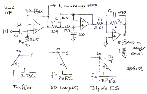
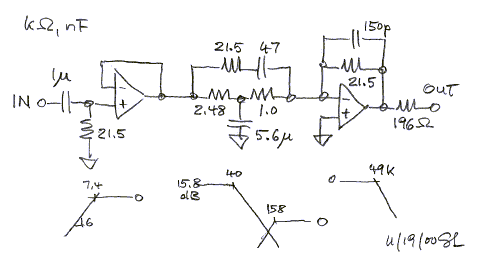
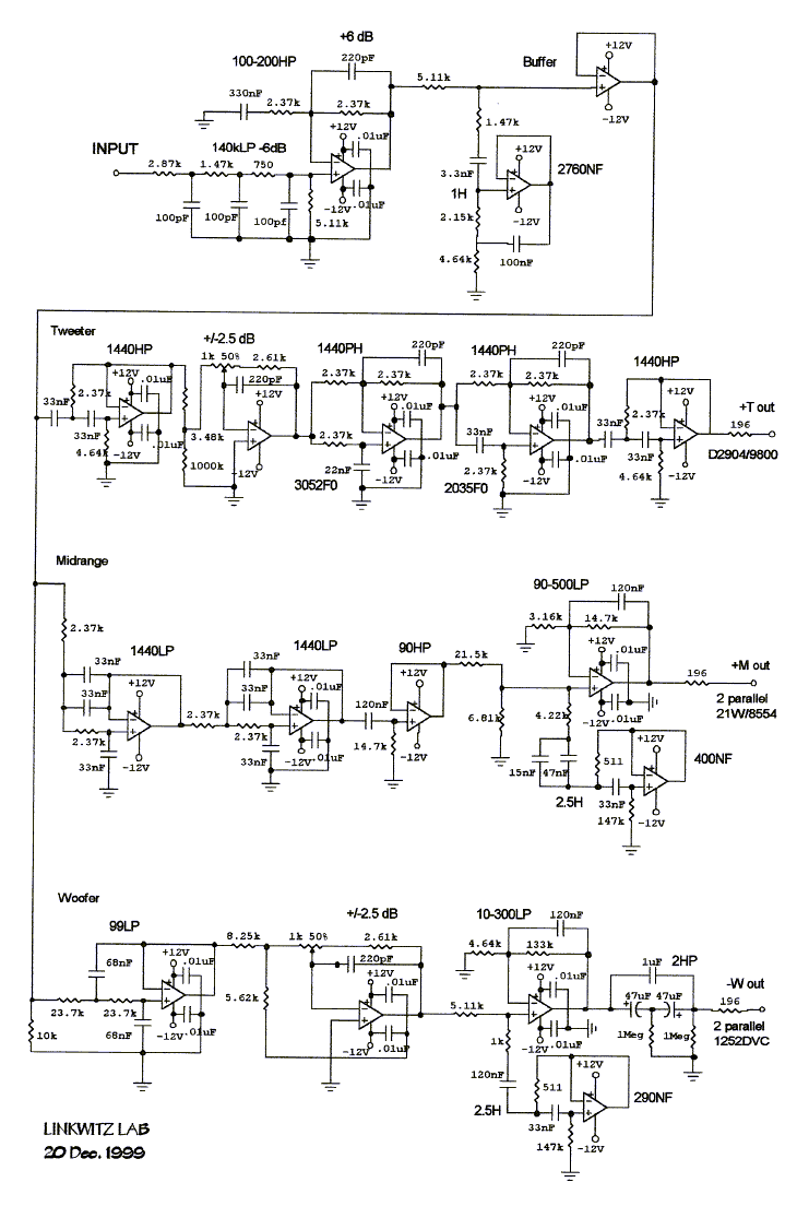
2 - 12 dB/oct Linkwitz-Riley crossover

The two outputs from the LR2 crossover filter are 180 degrees out of phase at all frequencies, which requires to use one of the drivers with reversed polarity, so that the two acoustic outputs add in phase. At the crossover frequency the filter outputs are 6 dB down.
The acoustic frequency and polar response is controlled by the electrical filters and the response of the mounted drivers. The electrical filter will not give the desired results, if there is insufficient overlap and flatness of the driver frequency response and when they are offset from each other. This can be corrected in many cases with the addition of a phase shift correcting network. I consider the crossover marginally useful, because the 12 dB/oct roll-off of the highpass filter below the crossover frequency does not reduce the excursions of a driver's cone when flat frequency response is obtained. My earlier assumption that the group delay of a 4th order LR4 crossover at low frequencies would introduce audible distortion was not correct. Therefore I recommend not to use the LR2 crossover. (38xo_eq1.gif, FAQ19, xo12-24b.gif)
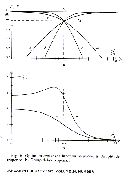
The LR2 circuit uses the Sallen-Key active filter topology to implement the 2nd order transfer function. The response is defined by w0 and Q0 which sets the location of a pole pair in the complex frequency s-plane and by an additional two zeros at s = 0 for the highpass filter. In the case of the LR2 filters Q0 = 0.5, and Q0 = 0.71 for each of the two cascaded 2nd order filters that form the LR4 filter. The frequency response is obtained by setting s = jw and solving the transfer function for magnitude and phase. The formulas below can be used to design filters with different values for w0 or Q0, or to analyze a given circuit for its w0 and Q0 values.
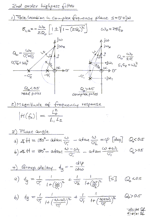


Any order Linkwitz-Riley filters can be implemented by a cascade of 2nd order Sallen-Key filters. The Q0 values for each stage are listed in the table below. The component values of each stage for a given crossover frequency f0 can be calculated by using Q0 and selecting a convenient value for C2 or R2 in the formulas above.
| LR2 | LR4 | LR6 | LR8 | LR10 | |
| Q0 of stage 1 | 0.5 | 0.71 | 0.5 | 0.54 | 0.5 |
| Q0 of stage 2 | 0.71 | 1.0 | 1.34 | 0.62 | |
| Q0 of stage 3 | 1.0 | 0.54 | 1.62 | ||
| Q0 of stage 4 | 1.34 | 0.62 | |||
| Q0 of stage 5 | 1.62 | ||||
| dB/octave slope | 12 | 24 | 36 | 48 | 60 |
Top
3 - 24 dB/oct Linkwitz-Riley crossover

The 24 dB/oct LR4 crossover filter provides outputs which are 360 degrees offset in phase at all frequencies. At the transition frequency Fp the response is 6 dB down. The electrical network will only give the targeted exact acoustic filter response, if the drivers are flat and have wide overlap. This is seldom the case. The steep filter slopes make the combined acoustic response less sensitive to magnitude errors in the driver responses, but phase shift errors usually have to be corrected with an additional allpass network. (xo12-24b.gif, 38xo_eq1.gif, models.htm#E) Top
 Russ Riley and Siegfried Linkwitz, September 2006, Douglas City, CA |
| In the
sixties,
early seventies, I
worked with Russ Riley at Hewlett-Packard's Palo Alto R&D laboratory
for the development of RF and Microwave test equipment. Like many other
engineers we had "G-Jobs", building such things as
electronic ignitions for our VW bugs and vans, FM receivers, phase-locked
pulse width FM demodulators, short-wave receivers, audio pre- and power
amplifiers, third octave audio analyzers, headphone equalizers, and of
course, loudspeakers. After measuring the acoustic and electrical
responses of commercial speakers we equalized them and tried to understand
why they were designed with strange looking driver layouts, used large
baffles, were stuffed with a variety of internal damping materials and
used various box stiffening and damping techniques. Eventually we
completely redesigned them and built our own speakers. Russ and his wife,
Vicky, an accomplished organist, always had the most critical and reliable ears. He
was an ingenious design engineer, a strong contributor, who inspired and
challenged many of us on our HP and unofficial design projects. Russ retired after over 40 years in R&D for HP/Agilent and now lives with his wife in a remote mountain valley, in a genuine log cabin, amongst pear, plum and walnut trees, berry bushes, chicken and deer, the sounds of a large creek, and the pine and fir trees that climb up the slopes. He died peacefully in his log cabin on December 6, 2010. |
4 - Delay correction

A first order allpass filter section with flat amplitude response but phase shift that changes from 0 degrees to -180 degrees, or -180 degrees to -360 degrees, is often used to correct phase response differences between drivers. Multiple sections may delay the tweeter output and compensate for the driver being mounted forward of the midrange. Active crossover circuits that do not include phase correction circuitry are only marginally useable. (allpass.gif, allpass2.gif, models.htm#E, 38xo_eq1.gif) Top
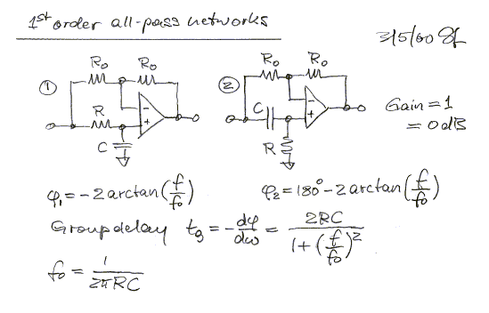
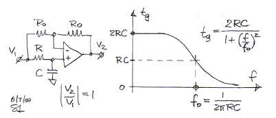
5 - Shelving lowpass

This type of circuit is useful to bring up the low frequency response in order to compensate for the high frequency boost from front panel edge diffraction. It can also serve to equalize the low frequency roll-off from an open baffle speaker. (shlv-lpf.gif, 38xo_eq1.gif) Top
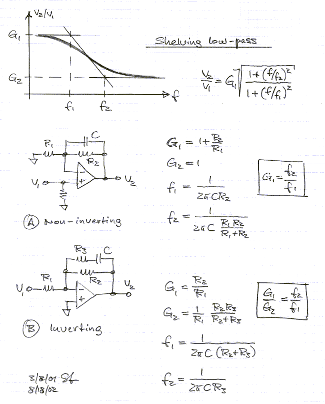
A passive RC version of the shelving lowpass is shown below.

6 - Shelving highpass

A circuit used to boost high frequencies or to smooth the transition between a floor mounted woofer and a free standing midrange. (shlv-hpf.gif, 38xo_eq1.gif, models.htm#F) Top
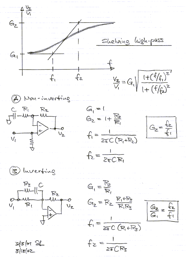
A passive RC version of the shelving highpass is shown below.

7 - Notch filter

Notch filters are used to introduce dips in the frequency response in order to cancel driver or room resonances. The three circuits above have the same response. A) is difficult to realize because of the large inductor. B) is used to remove the peak in the 6 dB/oct dipole response. C) gives convenient component values for room EQ below 100 Hz. (room EQ, inductr1.gif, inductr2.gif, 38xo_eq1.gif ) Top
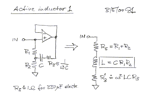
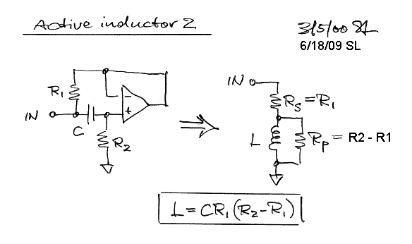

8 - 6 dB/oct dipole equalization

Equalization of the dipole frequency response roll-off usually requires not only a 6 dB/oct boost towards low frequencies, but also removal of a peak in the response. (Models A2) The three circuits differ in their ability to remove such peak.

A) The shelving lowpass filter cannot correct for a peak.
B) The bridged-T based circuit is limited in the shape of curves that can be realized. It has also higher gain for opamp noise than signal at high frequencies.
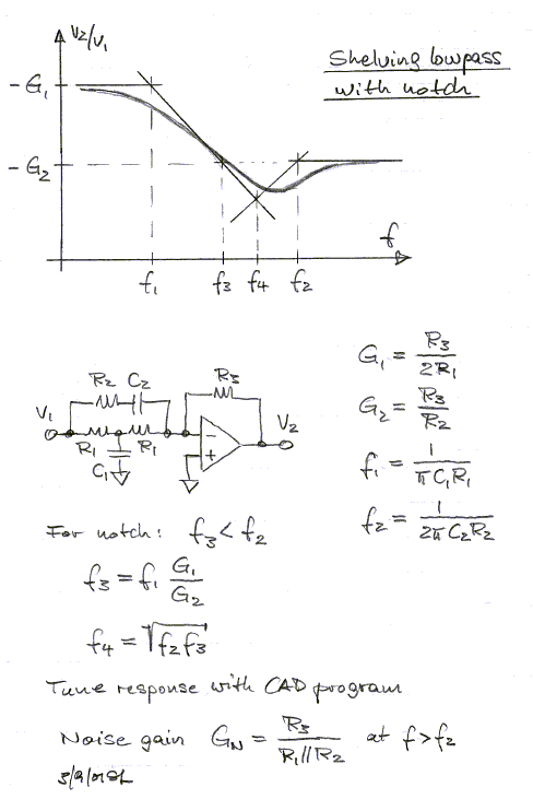
C) The shelving lowpass with added notch filter is the most flexible circuit. (models.htm#D) Top
9 - 12 dB/oct highpass equalization ("Linkwitz Transform", Biquad)

A majority of drivers exhibit second order highpass behavior because they consist of mechanical mass-compliance-damping systems. They are described by a pair of zeroes at the s-plane origin and a pair of complex poles with a location defined by Fs and Qt. The circuit above allows to place a pair of complex zeroes (Fz, Qz) on top of the pole pair to exactly compensate their effect. A new pair of poles (Fp, Qp) can then be placed at a lower or a higher frequency to obtain a different, more desirable frequency response.
This allows to extend the response of a closed box woofer to lower frequencies, in the above circuit example from 55 Hz to 19 Hz, provided the driver has adequate volume displacement capability and power handling. The equalizer frequency response is shown below, correcting for a woofer with peaked response (Qp = 1.21) and early roll-off (Fp = 55 Hz), to obtain a response that is 6 dB down at 19 Hz and with Q = 0.5 .

The associated phase and group delay responses are shown below.

Not only is the frequency response extended, but the time response is also improved, as indicated by the reduced overshoot and ringing of the lower cut-off highpass filter step response.

It can be seen from the s-plane description of the transfer functions that the complex poles of the driver in the box are canceled by a set of complex zeros in the equalizer. The specified real axis poles of the equalizer, together with the driver zeros at the s-plane origin, determine the overall loudspeaker response in frequency and time.

The equalizer action is difficult to visualize in the time domain, because the driver output waveform is the convolution of the input signal s(t) with the impulse response of the equalizer h1(t), which in turn must be convolved with the impulse response h2(t) of the driver. Convolution is a process whereby the current value of the time response is determined by the time weighted integral over past behavior. Below are the responses of driver, equalizer and driver-equalizer combination, if the input signal s(t) is an impulse.

More illustrative are the responses to a 4-cycle, rectangular envelope 70 Hz toneburst s(t). For example, the driver output is the convolution of the burst s(t) with the driver's impulse response h2(t). Note that the driver phase leads the input signal, as would be expected for a highpass response. Upon turn-off of the input burst at 57.14 ms the driver response rings towards zero, governed by Fp = 55 Hz and Qp = 1.21.

The equalizer output response lags its burst input. This signal will force upon the driver a response correction so that it is no longer dominated by Fp = 55 Hz and Qp = 1.21. The equalizer output signal is convolved with the impulse response h2(t) of the driver to obtain the desired equalized driver output. Now, the decay of the driver output follows the 2nd order highpass filter response determined by Qp = 0.5 and Fp = 19 Hz of the equalizer, after the excitation has stopped.
Of course, none of the driver mechanical parameters like mass, compliance and damping have been changed in the process of equalization, only the input signal to the driver has been modified.
The above circuit can also be used to correct the low frequency roll-off of a tweeter so that the equalized tweeter becomes a filter section in an exact LR4 acoustic highpass. (f0Q0fpQp.gif, pz-eql.xls, f0Q0.gif, FAQ15, sb80-3wy.htm, sb186-48.gif , sb186-50.gif)
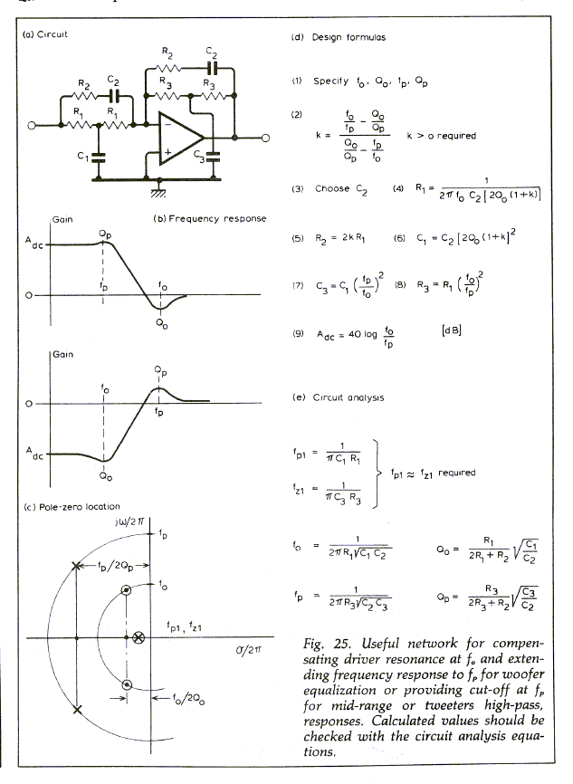
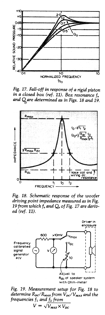
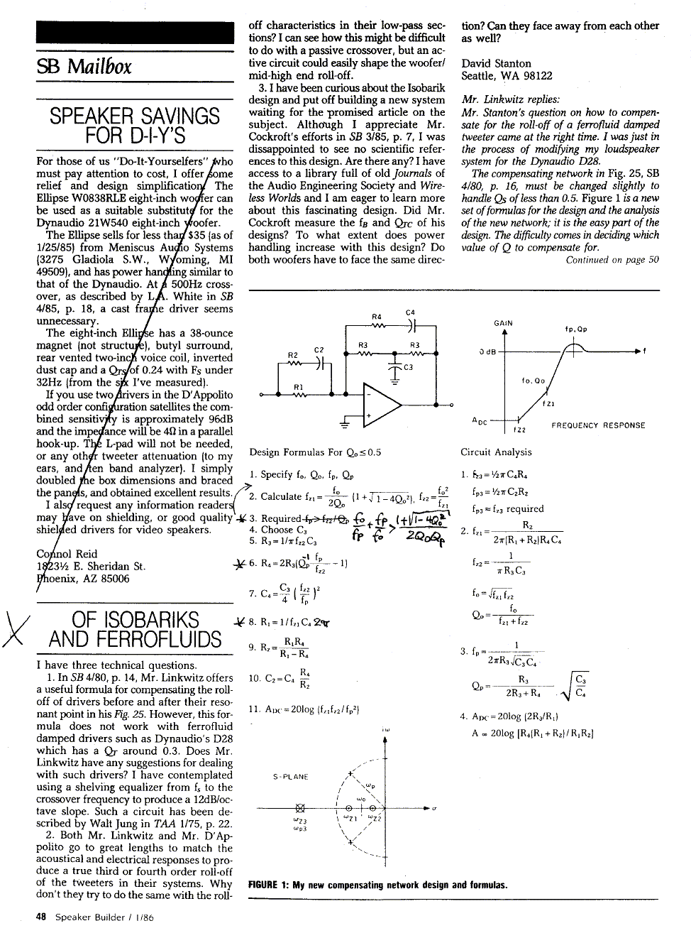

The 'CFL Linkwitz Transform Designer with Monte Carlo Sensitivity Ananlysis' by Charlie Laub makes component value selection easy and shows the effect of component tolerances upon the frequency response. Keep in mind that the LT is based on a measurement of driver parameters Fs and Qt. Only the small signal parameters are easy to define. Fs and Qt change with increasing signal level and to varying degree for different drivers. This makes the equalization imprecise, but it remains effective in practice.
Top
10 - Variable gain & fixed attenuation

A major advantage of line-level active crossovers is the efficiency with which drivers of different sensitivity can be combined in a speaker system. The three circuits use linear taper potentiometers but obtain a gain variation that is approximately linear in dB. Circuits B and C assume a 10k ohm load such as the input impedance of the power amplifier. Circuit A is optimal between filter stages because of its low output impedance. The placement of the variable gain stage in the filter chain must be carefully considered, because it affects noise performance and signal handling. (gain-adj.gif, attnrout.gif, 38xo_eq1.gif) Top
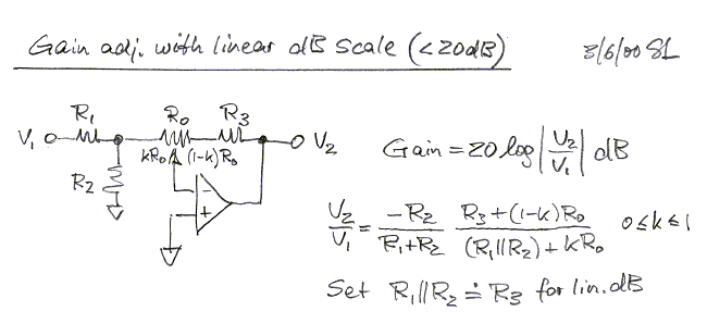
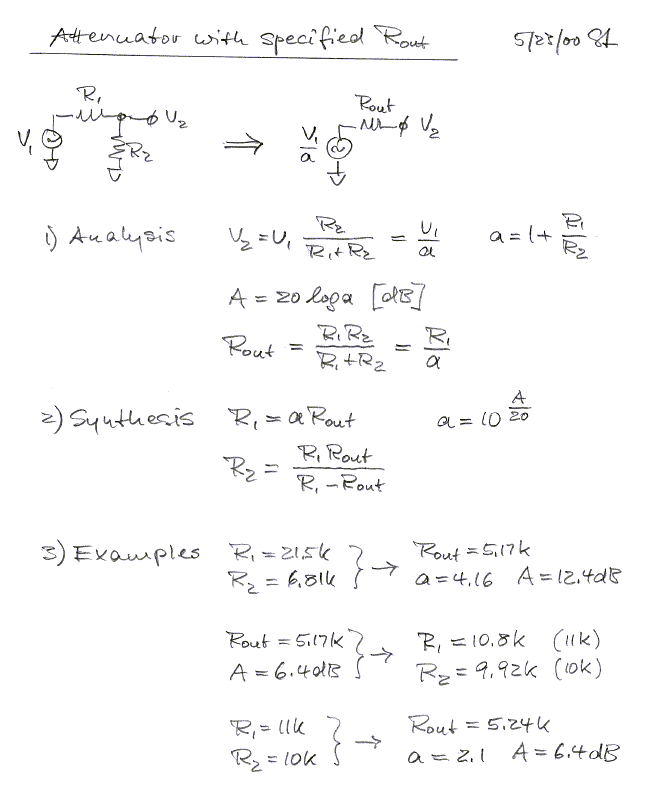
Occasionally a fixed attenuation of A dB or a is needed for the input voltage V2 of a circuit stage with input impedance R3 when driven from an operational amplifier with output voltage V1. In the example below a 3 dB (a=1.41) attenuation is desired. The load Rin that is seen by the opamp should be about 2000 ohm. The following amplifier stage has an input impedance of 10k ohm.

For designing an attenuator with specified output impedance Rout see: attnrout.gif
11 - Line driver

The output stage of the filter must be capable of driving cables, which typically have a capacitances in the order of 150 pF per meter length, without going into oscillation. A 196 ohm resistor maintains a resistive load component and tying output to negative input for out-of-band frequencies (>100 kHz) reduces loop gain. All of the above circuits can drive cables if operational amplifiers such as the OPA2134 or OPA2604 are used. In most cases it is not necessary to have a separate line driver.
Performance of active circuits should always be checked for inter-stage clipping, and for oscillation with a wideband (>10 MHz) oscilloscope. Top
12 - Power supply
I recommend to leave the effort of building a regulated power supply to one of the many vendors that offer wallplug and tabletop models. An output specification of +/-12 V to +/-15 V DC at >250 mA and with <1% ripple and noise will suffice. Often such supplies can be found at electronic surplus stores. Top13 - Printed circuit boards WM1 and MT1
To simplify the construction of active line-level equalizers and crossovers I offer three printed circuit boards, ORION/ASP, WM1 and MT1. The circuit traces are laid out to allow for a variety of filter designs. It is up to the user to determine the actual circuit configuration and component values. Then the necessary components and jumpers are loaded at the appropriate locations on the board to obtain the desired filter response. I will provide specific information for assembling the PHOENIX crossover/equalizer on the ORION/ASP pcb and a Linkwitz Transform on the WM1 pcb.WM1 is designed to implement the functionality of circuits 1, 5, 6, 7, 8, 9 or 10 and various combinations of these. The circuit board provides two of the topologies below for two channels of equalization or for a more elaborate single channel response correction.

The WM1 board can be used for:
- Equalization of an existing speaker with passive crossovers, baffle step correction and extension of the low frequency response.
- Pole-zero equalization of a closed box woofer and a LR2 crossover lowpass filter. Variable gain.
- Pole-zero equalization of a midrange and a LR2 crossover highpass filter.
- Dipole woofer equalization with notch and variable gain. LR2 crossover lowpass.
- Dipole woofer equalization for low Qts drivers.
- Low frequency, individual channel and overall response equalization of multi-way speakers, so long as elements of this topology allow you to generate the response you need.
- Equalization of add-on woofer , FAQ10, FAQ15
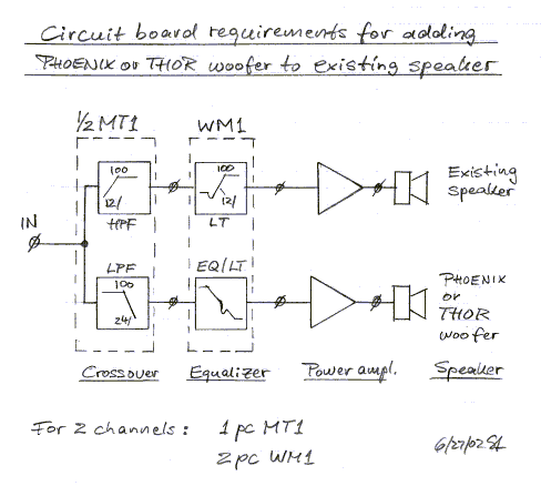
MT1 is designed to implement the functionality of circuits 1, 2, 3, 4, 5, 10 or 11 and various combinations of these. On the circuit board are two of the topologies below.

The MT1 board can be used to construct:
- A 2-way speaker with crossovers of order 1, 2, 3, or 4. The tweeter channel has variable gain and delay circuitry to align the tweeter's acoustic center with the woofer. The input buffer stage can provide 4p to 2p polar response (baffle step) correction.
- The tweeter and midrange channels of a 3-way system. The midrange highpass filter of the woofer to mid crossover would have to be provided by the WM1 board.
- The tweeter and upper midrange or upper midrange and lower midrange channels of a 4-way system.
- A great variety of active multi-channel line level filters in combination with the WM1 board.
- Crossover for add-on woofer, FAQ10, FAQ15
See the Circuit Board page for ordering information. Top
.
14 - Literature
Much useful information can be obtained from application notes of the various opamp manufacturers. If you need a refresher or an introduction to circuits, then read:[1] Martin Hartley Jones, A practical introduction to electronic circuits, Cambridge University Press, 1995. It is a well illustrated, easy to read, yet technically solid text. It covers a broad range of devices - from tubes to ICs - and many basic circuit functions.
The following books cover a range of concepts and go into depth on specific, relevant topics to strengthen understanding of electronic circuits and electro-acoustic models.
[2] Herman J. Blinchikoff & Anatol I. Zverev, Filtering in the Time and Frequency Domains, John Wiley, 1976. A broad and fundamental look at filters.
[3] Arthur B. Williams & Fred J. Taylor, Electronic Filter Design Handbook, McGraw-Hill, 1995. Design and analysis formulas for all types of filters.
[4] Jasper J. Goedbloed, Electromagnetic Compatibility, Prentice Hall,1990. Fundamental concepts and practices for dealing with radio frequency interference.
[5] Henry W. Ott, Noise Reduction Techniques in Electronic Systems, John Wiley, 1976. Practical steps to combat RFI.
[6] Manfred Zollner & Eberhard Zwicker, Elektroakustik, Springer, 1998. The most comprehensive and solid engineering level presentation of electro-acoustic transducers and related subjects.
In German, no comparable English language text available, to my knowledge.
[7] Walter G. Jung, editor, Op Amp Applications, Analog Devices, 2002. Everything you ever wanted to know about using operational amplifiers, and not just at audio frequencies.
Top
Suscribirse a:
Entradas (Atom)