Simply solving differential equations using Python, scipy and solve_ivp

https://medium.com/@bldevries/simply-solving-differential-equations-using-python-scipy-and-solve-ivp-f6185da2572d

Ben de Vries

·

Follow

6 min read

In this blog we will have a look at how we can use scipy and solve_ivp to numerically solve a second order ordinary differential equation (ODE). This is a very useful skill if you are in scientific visualization or any other technical discipline.

For example, I want to visualize black holes in a physics correct way. For this I am planning to solve the differential equations that govern how light travels in strong gravitational fields. Scipy and solve_ivp can help me do that numerically. But more on that in a later blog.

For now, we will take a simple differential equation that belongs to harmonic movement. If you are interested in some basic physics, read on, otherwise maybe skip the next section :)

This blog is part of a series, check out the next one also:

Prelude to chaos: solving non-linear differential equations with solve_ivp and scipy

Welcome to this blog where we will use solve_ivp and Python to solve a non-linear differential equation. Non-linear…

medium.com

Figure 1: drawing of a mass connected to a wall with a spring. When the mass gets a displacement x(t) from its equilibrium position (dashed vertical line) it will start oscillating about the equilibrium line. We assume the mass has no friction with the floor.

Newtons equations of motion for a harmonic oscillator

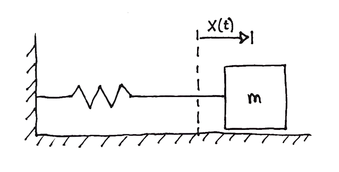
An example of a physical system that exhibits harmonic oscillations is a mass connected to a spring, see Fig. 1. Assuming no friction with the floor, if we displace the mass m from its equilibrium position and let it go, it will start to oscillate around its rest position. We can describe this movement with a differential equation using Newton’s equations of motion.

We assume that the force of the spring on the mass is proportional to the displacement (x(t)) and in the opposite direction to the displacement:

Eq. 1

Where k is the spring constant. The equation of motion now reads:

Eq. 2

And if we realize that the acceleration a is the second derivative of the displacement x:

Eq. 3

And this is the second order ordinary differential equation that we are going to solve using solve_ivp and scipy!

Exploring solve_ivp from the scipy package

Scipy has the great function solve_ivp which can integrate a system of ordinary differential equation for you. You can use it by calling:

scipy.integrate.solve_ivp(fun, t_span, y0)

The solve_ivp function can take more arguments but these three are necessary. Here fun stands for a Python function that implements the system of differential equations. And t_span is the range over which to integrate the differential equations. For example t_span=(0,1) integrates the system starting at 0 and up to 1. The last is y0 and this is a list of boundary conditions, one for every differential equation in the system.

Lets practice with solve_ivp and solve the simple differential equation for logarithmic functions:

Eq. 4

We now need to implement the right hand side of the differential equation into the function fun like this:

def fun(x, y):
  return -y

The function fun is given both the value of x and y for the current integration step. You then calculate the new value of dy/dx in fun(x,y) and return it.

We can solve the equation by first making a list of x values we want:

x_pts = np.linspace(0, 10, 11)

And then call solve_ivp over the interval x=0 to x=10 and using the boundary condition y(0)=1. We also use the t_eval argument to calculate the solution at the points in t_eval after the system is solved:

result = solve_ivp(fun, (0, 10), [1], t_eval=x_pts)

We can now print the result object and see that solve_ivp is succesfull:

message: The solver successfully reached the end of the integration interval.
success: True
status: 0
t: [ 0.000e+00 1.000e+00 2.000e+00 3.000e+00 4.000e+00
5.000e+00 6.000e+00 7.000e+00 8.000e+00 9.000e+00
1.000e+01]
y: [[ 1.000e+00 3.681e-01 1.355e-01 4.986e-02 1.835e-02
6.752e-03 2.486e-03 9.151e-04 3.370e-04 1.241e-04
4.572e-05]]
sol: None
t_events: None
y_events: None
nfev: 74
njev: 0
nlu: 0

We can now plot our solution together with the analytical solution y(x) = e^-x:

plt.plot(result.y[0,:], label = "Numerical solution")
plt.plot(x_pts, [math.e**(-x) for x in x_pts], "o", \
                label="Analytical solution")
plt.xlabel("x")
plt.ylabel("y(x)")
plt.legend()

And as you can see in Fig. 2 we have good agreement between the solution of solve_ivp and the analystical solution.

Figure 2: our numerical solution using solve_ipv and scipy of equation 4 (blue line) and the analytical solution (orange dots).

Solving our differential equation for harmonic motion using solve_ivp

Now it is time to solve our slightly more complicated differential equation describing harmonic motion. We will rewrite Eq. 3 as a system of coupled differential equations. We do this because the solve_ivp function does not take second order differential equations directly as an input. Now we can write (also setting k/m=1 to keep it simple):

Eq. 5

We now have two coupled functions to solve. In this example we can write the function fun as:

def fun(t, U):
  x, v = U
  return [v, -x]

Here U = [x(t), v(t)] and it is the current value of x(t) and v(t) that the integrator calculated and passed to fun(t, U). Now we must make sure the function returns the new value for [dx/dt, dv/dt] which is [v, -x] (see Eq. 5).

We can now calculate our solution like this:

U_0 = [0, 1]
t_pts = np.linspace(0, 15, 100)
result = solve_ivp(fun, (0, 20*math.pi), U_0, t_eval=t_pts)

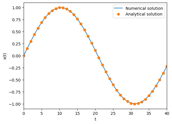
Here we have set our initial conditions to be x(0) = 0 and v(0) = 1. This will lead to a solution x(t) = sin(t). We plot our solutions in Fig.3.

plt.plot(result.y[0,:], label = "Numerical solution")
plt.plot([math.sin(t) for t in x_pts], "o", label="Analytical solution")
plt.xlabel("t")
plt.ylabel("x(t)")
plt.xlim(0,40)
plt.legend()

As you can see from Fig. 3, we have found the solution we expected!

Figure 3: our numerical solution using solve_ipv and scipy of equation 3 or 5 (blue line) and the analytical solution (orange dots).

In conclusion

We have solved the second order differential equation describing harmonic motion using solve_ivp, scipy and Python. You see it is not too difficult, its only tricky to translate the second order differential equation to two coupled first order equations that solve_ivp understands. I hope this blog gives you an idea on how to use solve_ivp, scipy and Python to solve your problem! Best of luck and see you in a next blog.