Windows 8.1 Lite V1 para Pc con bajos recursos 32 y 64 Bits

https://www.youtube.com/watch?v=e9RP0lvQ0Ic

https://www.youtube.com/watch?v=39APqRKkYpo

Como Instalar Windows 10 Pro Full En Español [2018]

Diseño de Filtros Activos y Pasivos - Design of Active and Passive Filters - Разработка активных и пассивных фильтров -

Diseño de Filtros Activos y Pasivos - Design of Active and Passive Filters - Разработка активных и пассивных фильтров -

http://www.analog.com/designtools/en/filterwizard/

http://sim.okawa-denshi.jp/en/Fkeisan.htm


http://axotron.se/blog/tool-for-designing-butterworth-and-chebyshev-filters/

Filter Design and Analysis

This page is the index of web calculator that design and analysis analog filters.

RC Filters

Vin(s)→

→Vout(s)

RC Low-pass Filter Tools
[Sample calculation]
[Sample calculation for PWM]

Vin(s)→

→Vout(s)

RC High-pass Filter Tools
[Sample calculation]

LR Filter

Vin(s)→

→Vout(s)

LR Low-pass Filter Tools
[Sample calculation]
[Sample calculation for PWM]

Vin(s)→

→Vout(s)

LR High-pass Filter Tools
[Sample calculation]

RLC Filter

Vin(s)→

→Vout(s)

RLC Low-pass Filter Tools
[Sample calculation]

Vin(s)→

→Vout(s)

RLC High-pass Filter Tools
[Sample calculation]

Vin(s)→

→Vout(s)

RLC Band-pass Filter Tools
[Sample calculation]

Vin(s)→

→Vout(s)

RLC Band-stop Filter Tools
[Sample calculation]

Sallen-Key Active Filter

Sallen-Key Low-pass Filter Tools
[Sample calculation]

Sallen-Key High-pass Filter Tools
[Sample calculation]

3rd order Sallen-Key Low-pass Filter Tools
[Sample calculation]

3rd order Sallen-Key High-pass Filter Tools
[Sample calculation]

Multiple feedback Active Filter

Multiple feedback Low-pass Filter Tools
[Sample calculation]

Multiple feedback High-pass Filter Tools
[Sample calculation]

Multiple feedback Band-pass Filter Tools
[Sample calculation]

3rd order Multiple feedback Low-pass Filter Tools
[Sample calculation]

3rd order Multiple feedback High-pass Filter Tools
[Sample calculation]

Twin-T Notch Filter

Twin-T Notch Filter Tools
[Sample calculation]

2nd order CR filter

2nd order CR filter Tools
[Sample calculation]

Tool for designing Butterworth and Chebyshev filters

2016-03-05Electronics, PC

Designing passive LC-filters typically involves looking up prototype filter component values in a table in reference books like “Handbook of Filter Synthesis” by Zverev or “Design of Microwave Filters, Impedance-Matching Networks, and Coupling Structures” by Matthaei et. al., then transforming the values to produce a filter with the desired impedance and cut-off frequency. This can be a bit tedious and error prone, so when I found out about the classic Matthaei book, which is downloadable via the link above, and that it contains the math required to calculate the prototype filter component value tables, I set out to create a spreadsheet to help with the filter design.

In addition to calculating the (previously) magical prototype tables for Butterworth and Chebyshev (with user-specified pass-band ripple) filters, the spreadsheet also performs the frequency and impedance transformation for filters of orders from 1 to 10.

To make the design process even quicker and better, I added a feature to create LTSpiceschematics of the selected filter so that the filter properties can be simulated (and perhaps manually adapted to standard component values and to include parasitics) using LTSpice. I used the SI prefix formatting function I wrote about in the previous blog post to write out the component values in a pretty manner.

The usage of the spreadsheet should be fairly self-explanatory, but there are also usage instructions on the first tab. Basically, the user should fill out the values in yellow cells and leave the rest alone. I did not lock any cells, since I often get annoyed by spreadsheets with locked cells and I encourage others to modify and improve it.

Here is a link to the Excel 2002 file:

 FilterSynthesis_v1.0.xls

Make sure that macros are enabled if you want to use the LTSpice export features.

Here are some screenshots

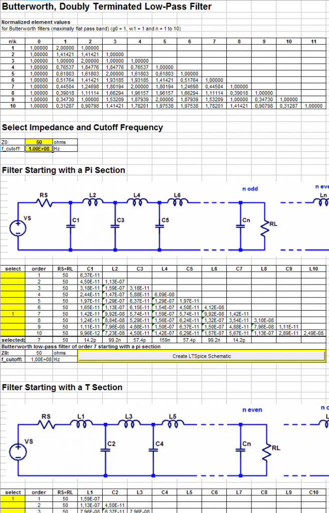
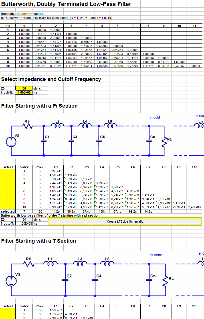
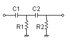
Butterworth tab

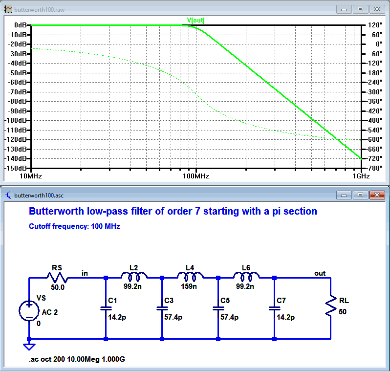
LTSpice simulation of a Butterworth schematic generated by the spreadsheet.

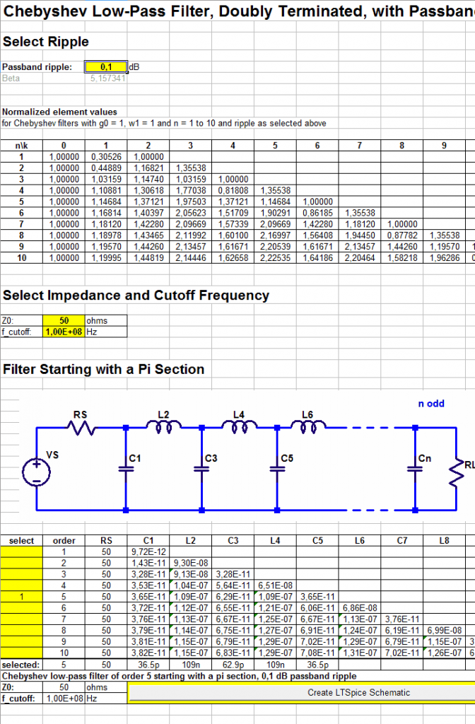
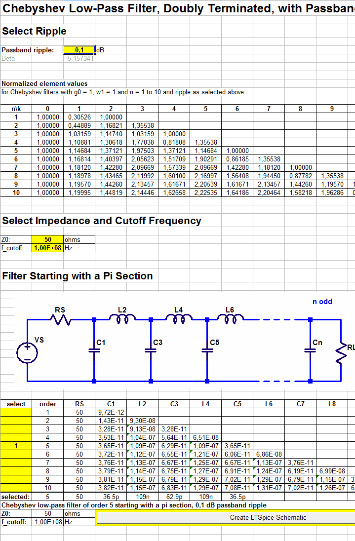
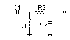
Chebyshev tab

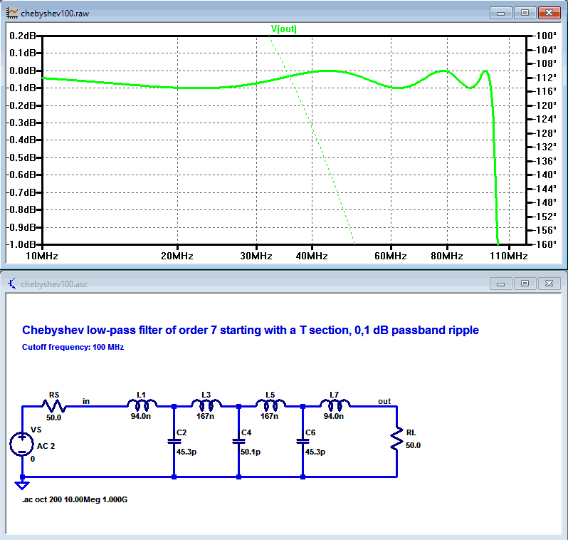
LTSpice simulation of a Chebyshev schematic generated by the spreadsheet.

Practical Numerical Methods with Python MAE 6286

Start Date:Sep 1, 2017

Duration:15 weeks

Price:Free

https://openedx.seas.gwu.edu/courses/course-v1:MAE+MAE6286+2017/about

Course Description

This is a first course in numerical methods for advanced students in engineering and applied science. It was developed in 2014, both as a massive open online course (MOOC) and a regular course at the George Washington University. Similar courses have been taught at partner institutions: Southampton University (UK), Pontifical Catholic University of Chile, and Université Libre de Bruxelles. The original MOOC instance stayed online until August 2017, reaching 8,280 registered users. This is a refreshed instance of the course, as the GW SEAS Open edX has been re-installed with the latest version of the software in August 2017. Users of the old site can access with their same login credentials, but course enrollments were not kept—please enroll again if you are still interested in this course!

What You'll Learn

• Connect the physics represented by a mathematical model to the characteristics of numerical methods to be able to select a good solution method
• Implement a numerical solution method in a well-designed, correct computer program
• Interpret the numerical solutions that were obtained in regards to their accuracy and suitability for applications

Instructors

Lorena A. BarbaAssociate Professor of Mechanical and Aerospace EngineeringThe George Washington University

Prof. Bernard KnaepenProfessor of PhysicsUniversité Libre de Bruxelles

Dr. Ian HawkeLecturer of MathematicsSouthampton University

Course Outline

Expand All

Minimize All

1. Getting Started 
   1. Initial Survey 
      1. Country survey
      2. Geochart of participants
      3. Survey
   2. How is this course going to work? 
      1. What to expect from the instructors
      2. What is expected of you
      3. What are the connected courses?
      4. What's this course about?
   3. Course communication channels 
      1. Discussion board
      2. Twitter
      3. Gitter chat room
   4. Why Python? 
      1. Python is a good learning language
      2. Python can get you a job
      3. An HPC expert uses Python
      4. Why Python tweet-up
   5. Are you new to Python? The basics. 
      1. For total beginners
      2. For beginners: quiz
      3. Python Libraries
      4. Variables
      5. Whitespace in Python
      6. Conditionals and Functions
      7. Defining functions
      8. Slicing arrays
      9. Boolean Logic
      10. Copying vs. Pointing
      11. New to Python: quiz
   6. Get Python 
      1. How to work with Python on the cloud
      2. How to get Python on your computer
   7. Ways to get help 
      1. StackOverflow
      2. Anaconda help
   8. Jupyter notebooks 
      1. How to launch the Jupyter notebook
      2. How to execute code in the Jupyter notebook
      3. How to use Markdown in the Jupyter notebook
      4. Extra tips with the Jupyter notebook
   9. What's git and why do I need it? 
      1. Version Control
      2. Why do I need this?
      3. How does version control work?
      4. Quiz: version control
   10. Using git and GitHub 
       1. Getting started with GitHub
       2. git setup
       3. Configuring a git editor
       4. Creating a git repository
       5. Making your first commit
       6. Editing a tracked file
       7. Viewing a repo's history
       8. Uploading your repository to GitHub
       9. "Why GitHub?" tweet chat
   11. Downloading (cloning) the notebooks 
       1. Forking the Numerical-MOOC Repository
       2. Making your first commit to your fork
   12. Self-Assessment checklist 
       1. Self-assessment purpose and surveys
       2. New to Python
       3. Get Python
       4. New to GitHub
2. Module 1: The Phugoid Model 
   1. Introduction. Phugoid theory 
      1. Introduction
      2. Lanchester's "Aerodonetics"
   2. Module 1 graded assessment 
      1. Tools of scientific Python
      2. Numerical solution of initial value problems
      3. Coding assignment: Rocket flight
   3. Dig deeper: Euler's method and beyond 
      1. Euler's method is a first order method
3. Module 2: Space and Time 
   1. Introduction to finite-difference solution of PDEs 
      1. Jupyter Notebooks
   2. Module 2 graded assessment 
      1. Stencils
      2. Numerical Solutions
      3. Coding Assignment: Traffic Flow
   3. Dig deeper: Analysis of numerical schemes 
      1. Analysis of schemes
4. Module 3: Riding the Wave 
   1. Riding the wave: Convection problems 
      1. IPython Notebooks
      2. Schemes for convection
      3. References
   2. Practice with Burgers' equation 
      1. Burgers with MacCormack
      2. Add damping
   3. Module 3 graded assessment 
      1. Flux limits
      2. Taylor Time
      3. Coding Assignment: Sod's Shock Tube
5. Module 4: Spreading Out 
   1. Spreading out: diffusion problems 
      1. Jupyter Notebooks
      2. Boundary conditions
   2. Module 4 graded assessment 
      1. Boundary Conditions
      2. Coding Assignment: Reaction-DIffusion
6. Module 5: Relax and Hold Steady 
   1. Relax and hold steady: elliptic problems 
      1. Module 5 Jupyter Notebooks
      2. Iterative solvers
   2. Module 5 graded assessment 
      1. Iterative Methods
      2. Coding Assignment: Stokes Flow