lunes, 28 de noviembre de 2022

Create an inventory management app from Google Sheets with AppSheet

https://blog.google/products/google-cloud/how-to-build-an-inventory-management-apps-no-coding-necessary/


Create an inventory management app from Google Sheets with AppSheet


Google Cloud’s AppSheet lets you create apps without writing a line of code. From managing to-do lists to tracking your dog’s habits, you can now create apps to simplify your life. 

We often see people building inventory management apps, whether it’s to run a large retail business or just to sell products as a side job. Normally, tracking inventory can be difficult, especially if you’re doing it in a spreadsheet or database. With AppSheet, however, you can make inventory tracking much simpler by building your own tailored inventory management app.

In this post, we’ll show you how you can build an inventory management application with AppSheet in a few steps. The app we’ll create will include the following features:

  •  Use barcode scanners to record stock in and stock out

  • Automatically calculate current stock level

  • Display what items need to be restocked

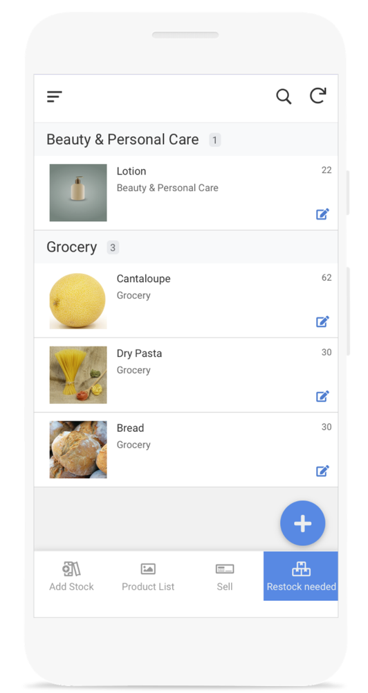
We’ve already built this app, so if you want to use it to follow along or start using it now, you can access it here. Here’s a look at the app:

appsheet

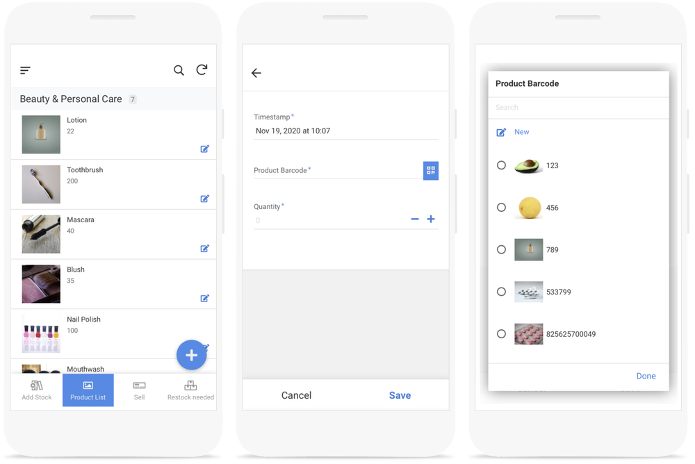
Let’s build your inventory management app.

Step 1: Organize your data and generate your app

AppSheet apps connect to data sources, such as Google Sheets. But before connecting your data to AppSheet, you’ll want to make sure it’s set up appropriately. Set up your data with column headers in the first row, and rows of data underneath. 

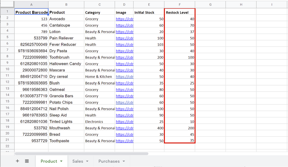
To set up the data for this app, we created three tables in a Google Sheet (that you can copy here):

  • “Product” for all product information

  • “Sales” for items sold or removed out from stock;

  • “Purchases” for products added to stock.

Now, let’s turn this data into an app. If you’re in Google Sheets, you can go to Tools>AppSheet>Create an App, and AppSheet will convert your data into an AppSheet app.

Tools>AppSheet>Create an App

AppSheet will automatically add one of your data tables to your app. You can add the other tables by going to Data>Tables>Add a table.

AppSheet will automatically add one of your data tables to your app. You can add the other tables by going to Data>Tables>Add a table.

It’s also created a view for you, showing the Products. You can create additional views for the other tables by going to UX>Views, select New View, name your view, and set the view type to form. We’ll call our views Product List, Sell, and Add Stock.

It’s also created a view for you, showing the Products. You can create additional views for the other tables by going to UX>Views, select New View, name your view, and set the view type to form. We’ll call our views Product List, Sell, and Add Stock.

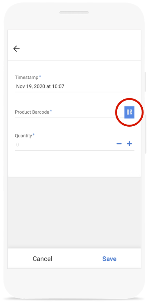
Step 2: Set up the barcode scanner

AppSheet can use the camera on your mobile device to capture barcoded data. To do this: Go to Data>Columns in the AppSheet Editor and mark the “Product Barcode” column in both the “Purchases” and “Sales” tables as searchable and scannable.

Set up the barcode scanner

Your app is now ready to record any inventory movement, whether it is stock in or stock out. All you have to do is to tap on the barcode scanner button (under “Add Stock” or “Sell” view) and scan the item.

barcodesettings

Step 3: Calculate the real-time inventory level

We want to see the current inventory level of each item in our app. The calculation formula is pretty simple: 

Current stock level = initial stock + stock in – stock out

To set it up, the first step is to configure our app to automatically record real-time inventory levels. You can do this by linking the data in the tables together. Since every table includes a column for the product barcode numbers, use that data to link the apps.

We’ll connect our Product Barcode columns in the “Sales” and “Purchases” sheets with the Product Barcode column in the Product sheet. To do this: Go to Data>Columns> Sales, and click on Product Barcode and edit the column definition by following the three steps below:

  1. Name the Column “Product Barcode”

  2. Select Ref on the Type drop-down list

  3. Select Products as ReferencedTableName

Calculate the real-time inventory level

Then repeat these same steps for the Purchases table.

Now let’s tell our app how to calculate the inventory level! Go to Data>Columns and in the “Products” table select Add virtual column. Add this app formula in the popup box:

COUNT([Related Purchases]) - COUNT([Related Sales]) + [Initial Stock].

how to calculate the inventory level

And that’s it. If you go to UX>View>Product List view, you can select either the Deck view or Table view, then select Current Stock as one of your headers. You will see every product’s Current Stock level.

And that’s it. If you go to UX>View>Product List view, you can select either the Deck view or Table view, then select Current Stock as one of your headers. You will see every product’s Current Stock level.

Step 4: Display “Restock Needed” for low inventory products

Inventory managers need to make sure there is enough inventory to sell and that shelves are full. This final step will set up a view that shows which items need to be restocked.

1. Set a restock level for every product. This will likely be different for each product. To determine the right number, you can review historical data and check out your demand forecast.

Display “Restock Needed” for low inventory products

2. Create a slice. Go to Data>Slices, select Create a slice and name it “Restock Needed.” Set the Source Table as Product and the Row Filter Condition to be: [Current Stock] <= [Restock Level]. This formula says, “Give me the data if a product’s Current Stock level is lower than or equal to Restock Level.”

Row Filter Condition

3. Create a view for the slice. Go to UX>Views and select New View. Choose Restock Needed (slice) as your data source, and choose the view type you want (we went with the deck view type).

Create a view for the slice

Now we can see all the products that need to be restocked.

Now we can see all the products that need to be restocked.

Congratulations, you now have a working inventory management app! From here you can customize it and add additional functionality, such as email notificationsthemes, and new views. If you ran into any issues building your app, check out our help articles or ask a question on the AppSheet Community

Chebyshev Approximation and How It Can Help You Save Money, Win Friends, and Influence People

https://www.embeddedrelated.com/showarticle/152.php

Chebyshev Approximation and How It Can Help You Save Money, Win Friends, and Influence People


CHEBYSHEV POLYNOMIALS

The key to using polynomials to evaluate functions, is not to think of polynomials of being composed of linear combinations of 1,x,x2,x3, etc., but as linear combinations of Chebyshev polynomials Tn(x). As discussed in more detail in the Wikipedia page, these have the following special properties:

  • they are minimax functions over the range [1,1], e.g. all their minima/maxima/extrema are at ± 1 (see diagram below)
  • they are orthogonal over the range [1,1] with weight 11x2
  • T0(x)=1,T1(x)=x,Tn+1(x)=2xTn(x)Tn1(x)
  • Tn(x)=cos(ncos1x)

Figure: Chebyshev functions Tn(x), courtesy of Wikipedia

Let's say we have a given function f(x) over the range x[a,b]. We can express f(x)=ckTk(u) where u=2xabba and x=ba2u+a+b2, which is a transformation which maps the interval x[a,b] to u[1,1]. The problem then becomes a matter of figuring out the coefficients ck, which can be done using the Chebyshev nodes:

These are easier to understand graphically; they are merely the projections onto the x-axis of the midpoints of equal interval circular arcs of a semicircle:

You will note that the nodes are spaced equally near 0 and more compressed towards ± 1.

To approximate a function by a linear combination of the first N Chebyshev polynomials (k=0 to N-1), the coefficient ck is simply equal to A(k) times the average of the products Tk(u)f(x) evaluated at the N Chebyshev nodes, where A=1 for k=0 and A=2 for all other k.

Let's illustrate the process more clearly with an example.

Suppose f(x)=13x3+2x2+x10 over the range [1,3], with u=x12,x=2u+1:

Let's use N=5. The Chebyshev nodes for N=5 are u=0.951057,0.587785,0,+0.587785,+0.951057. This corresponds to x=0.902113,0.175571,1,2.175771,2.902113, and the function f(x) evaluated at those nodes are y=9.51921,10.11572,6.66667,5.07419,17.89408.

For c0 we compute the average value of y = (9.5192110.115726.66667+5.07419+17.89408)/5=0.66667.

For c1 we compute 2 × the average value of u × y = 2×(9.51921×0.951057+10.11572×0.587785 +6.66667×0+5.07419×0.587785+17.89408×0.951057)=14

For c2 we compute 2 × the average value of T2(u)×y=(2u21)×yc2=6

For c3 we compute 2 × the average value of T3(u)×y=(4u33u)×yc3=0.66667

For c4 we compute 2 × the average value of T4(u)×y=(8u48u2+1)×yc4=0

The conclusion here is that f(x)=23T0(u)+14T1(u)+6T2(u)+23T3(u) ; if you go and crunch through the algebra you will see that the result is the same as f(x)=13x3+2x2+x10.

So what was the point here....? Well, if you already have the coefficients of a polynomial, there's no point in using Chebyshev polynomials. (If the input range is significantly different from [1,1], a linear transformation from x to u where u[1,1] will give you a polynomial in u that has better numerical stability, and Chebyshev polynomials are one way to do this transformation. More on this later) If you want to approximate the polynomial with a polynomial of lesser degree, Chebyshev polynomials will give you the best approximation.

For example let's use a quadratic function to approximate f(x) over the input range in question. All we need to do is truncate the Chebyshev coefficients: let's computef2(x)=23T0(u)+14T1(u)+6T2(u)=23+14u+6×(2u21)=203+14u+12u2=203+7(x1)+3(x1)2=3x2+x323.

Voila! We have a quadratic function that is close to the original cubic function, and the magnitude of the error is just the coefficient of the Chebyshev polynomial we removed = 23.

You will note that these two polynomials (13x3+2x2+x10 and 3x2+x323), expressed in their normal power series form, have no obvious relation to each other, whereas the Chebyshev coefficients are the same except in coefficient c3 which we set to zero to get a quadratic function.

In my view, this is the primary utility of expressing a function in terms of its Chebyshev coefficients: The coefficient c0 tells you the function's average value over the input range; c1 tells you the function's "linearness", c2 tells you the function's "quadraticness", c3 tells you the function's "cubicness", etc.

Here's a more typical and less trivial example. Suppose we wish to approximate log2x over the range [1,2].

A decomposition into Chebyshev coefficients up to degree 6 yields the following:

c0=+0.54311c1=+0.49505c2=0.042469c3=+0.0048577c4=6.2508×10⁴c5=+8.5757×10⁵c6=1.1996×10⁵


You will note that each coefficient is only a fraction of the magnitude of the previous coefficient. This is an indicator that the function in question (over the specified input range) lends itself well to polynomial approximation. If the Chebyshev coefficients don't decrease significantly by the 5th coefficient, I would classify that function as "nonpolynomial" over the range of interest.

The maximum error for the 6th-degree Chebyshev approximation for log2x over x[1,2] is only about 2.2×10⁻⁶, which is approximately the value of the next Chebyshev coefficient.

If we truncate the series to a 4th-degree Chebyshev approximation, we get a maximum error that is about equal to c5=8.6×10⁵: