https://homepage.stat.uiowa.edu/~mbognar/1030/Bickel-Berkeley.pdf
sábado, 17 de diciembre de 2022
paradoja de Simpson - En 1973, la Universidad de California, Berkeley tenía algunas preocupaciones sobre las admisiones de estudiantes a sus cursos de posgrado
En 1973, la Universidad de California, Berkeley tenía algunas preocupaciones sobre las admisiones de estudiantes a sus cursos de posgrado
El cuento de precaución de la paradoja de Simpson
1.2: El cuento de precaución de la paradoja de Simpson


- Última actualización

La siguiente es una historia real (creo que...). En 1973, la Universidad de California, Berkeley tenía algunas preocupaciones sobre las admisiones de estudiantes a sus cursos de posgrado. Específicamente, lo que causó el problema fue que el desglose por género de sus admisiones, que se veían así...
| Número de aspirantes | Porcentaje admitido | |
|---|---|---|
| Machos | 8442 | 46% |
| Hembras | 4321 | 35% |
... y los estaban preocupados por ser demandados. 4 Dado que había cerca de 13 mil aspirantes, una diferencia de 9% en las tasas de admisión entre hombres y mujeres es demasiado grande para ser una coincidencia. Datos bastante convincentes, ¿verdad? Y si te dijera que estos datos reflejan en realidad un sesgo débil a favor de las mujeres (¡más o menos!) , probablemente pensarías que yo era una locura o sexista.
Curiosamente, en realidad es cierto... cuando la gente empezó a mirar más cuidadosamente los datos de admisiones (Bickel, Hammel y O'Connell 1975) contaban una historia bastante diferente. Específicamente, cuando lo miraron departamento por departamento, resultó que la mayoría de los departamentos en realidad tenían una tasa de éxito ligeramente mayor para las aspirantes femeninas que para las aspirantes masculinas. En el cuadro 1.1 se muestran las cifras de admisión para los seis departamentos más grandes (con los nombres de los departamentos eliminados por razones de privacidad):
Cuadro 1.1: Cifras de admisión para los seis departamentos más grandes por género
| Departamento | Solicitantes Masculinos | Porcentaje Masculino Admitido | Solicitantes Femeninas | Porcentaje de mujeres admitidas |
|---|---|---|---|---|
| A | 825 | 62% | 108 | 82% |
| B | 560 | 63% | 25 | 68% |
| C | 325 | 37% | 593 | 34% |
| D | 417 | 33% | 375 | 35% |
| E | 191 | 28% | 393 | 24% |
| F | 272 | 6% | 341 | 7% |
Sorprendentemente, ¡la mayoría de los departamentos tuvieron una mayor tasa de ingresos para las mujeres que para los hombres! Sin embargo, la tasa general de ingreso en la universidad para las mujeres fue menor que para los hombres. ¿Cómo puede ser esto? ¿Cómo pueden ser veraces ambas afirmaciones al mismo tiempo?
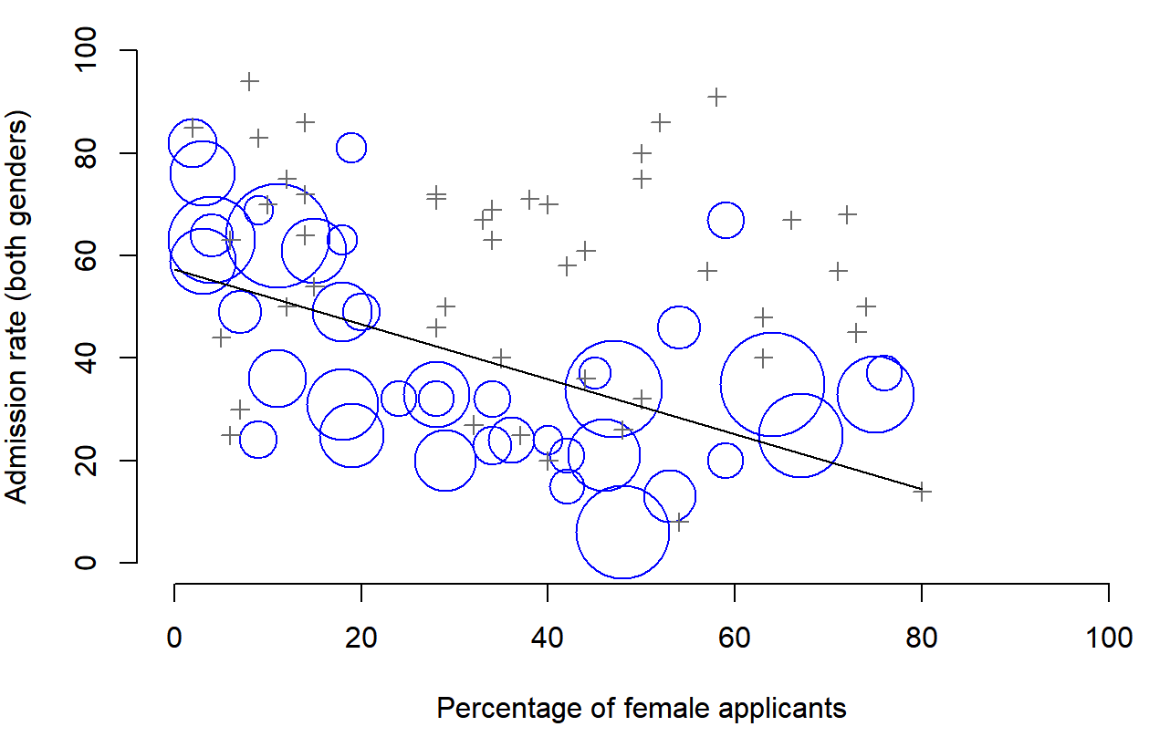
Esto es lo que está pasando. En primer lugar, observe que los departamentos no son iguales entre sí en términos de sus porcentajes de admisión: algunos departamentos (por ejemplo, ingeniería, química) tendían a admitir un alto porcentaje de los aspirantes calificados, mientras que otros (por ejemplo, el inglés) tendían a rechazar la mayoría de los candidatos, aunque fueran de alta calidad. Entonces, entre los seis departamentos arriba indicados, observe que el departamento A es el más generoso, seguido por B, C, D, E y F en ese orden. A continuación, observe que machos y hembras tendían a postularse a diferentes departamentos. Si clasificamos los departamentos en términos del número total de aspirantes masculinos, obtenemos A > B>D>C>F>E (los departamentos “fáciles” están en negrita). En conjunto, los varones tendían a postularse a los departamentos que tenían altas tasas de ingreso. Ahora compara esto con cómo se distribuyeron las aspirantes femeninas. La clasificación de los departamentos en términos del número total de mujeres aspirantes produce un ordenamiento bastante diferente C>E>D>F> A > B. Es decir, lo que estos datos parecen sugerir es que las aspirantes solían postularse a departamentos “más duros”. Y de hecho, si nos fijamos en toda la Figura 1.1 vemos que esta tendencia es sistemática, y bastante llamativa. Este efecto se conoce como la paradoja de Simpson. No es común, pero sí sucede en la vida real, y la mayoría de las personas se sorprenden mucho cuando lo encuentran por primera vez, y muchas personas se niegan incluso a creer que es real. Es muy real. Y si bien hay muchas lecciones estadísticas muy sutiles enterradas ahí, quiero usarla para hacer un punto mucho más importante... investigar es difícil, y hay muchas trampas sutiles y contradictorias que acechan a los incautos. Esa es la razón #2 por qué a los científicos les encantan las estadísticas, y por qué enseñamos métodos de investigación Porque la ciencia es dura, y la verdad a veces se esconde astutamente en los rincones y recovecos de datos complicados.
Antes de dejar este tema por completo, quiero señalar algo más realmente crítico que a menudo se pasa por alto en una clase de métodos de investigación. La estadística solo resuelve parte del problema. Recuerden que iniciamos todo esto con la preocupación de que los procesos de admisión de Berkeley pudieran estar injustamente sesgados contra las aspirantes femeninas. Cuando miramos los datos “agregados”, sí parecía que la universidad discriminaba a las mujeres, pero cuando “desagregamos” y miramos el comportamiento individual de todos los departamentos, resultó que los departamentos reales estaban, en todo caso, ligeramente sesgados a favor de las mujeres. El sesgo de género en las admisiones totales se debió a que las mujeres tendían a autoseleccionar para departamentos más duros. Desde una perspectiva jurídica, eso probablemente pondría a la universidad en claro. Las admisiones de posgrado se determinan a nivel del departamento individual (y hay buenas razones para hacerlo), y a nivel de departamentos individuales, las decisiones son más o menos imparciales (el sesgo débil a favor de las mujeres en ese nivel es pequeño, y no consistente entre departamentos). Dado que la universidad no puede dictar a qué departamentos la gente elige postularse, y la toma de decisiones se lleva a cabo a nivel del departamento, difícilmente se le puede responsabilizar de los sesgos que esas elecciones produzcan.
Esa fue la base de mis comentarios algo simples antes, pero esa no es exactamente toda la historia, ¿verdad? Después de todo, si nos interesa esto desde una perspectiva más sociológica y psicológica, podríamos preguntarnos por qué existen diferencias de género tan fuertes en las aplicaciones. ¿Por qué los hombres tienden a aplicar a la ingeniería con más frecuencia que las mujeres, y por qué esto se invierte para el departamento de inglés? ¿Y por qué ocurre que los departamentos que tienden a tener un sesgo de solicitud femenina tienden a tener tasas de admisión generales más bajas que aquellos departamentos que tienen un sesgo de solicitud masculina? ¿Podría esto no reflejar todavía un sesgo de género, a pesar de que cada departamento es imparcial en sí mismo? Podría. Supongamos, hipotéticamente, que los varones prefirieron aplicar a las “ciencias duras” y las mujeres prefieren las “humanidades”. Y supongamos además que la razón por la que los departamentos de humanidades tienen bajas tasas de admisión es porque el gobierno no quiere financiar las humanidades (los lugares de doctorado, por ejemplo, suelen estar vinculados a proyectos de investigación financiados por el gobierno). ¿Eso constituye un sesgo de género? ¿O simplemente una visión poco iluminada del valor de las humanidades? Y si alguien de alto nivel en el gobierno recortara los fondos de humanidades porque sintieran que las humanidades son “cosas inútiles de pollito”. Eso parece bastante descaradamente sesgado de género. Nada de esto entra en el ámbito de la estadística, pero es importante para el proyecto de investigación. Si estás interesado en los efectos estructurales generales de los sesgos sutiles de género, entonces probablemente quieras mirar tanto los datos agregados como los desagregados. Si estás interesado en el proceso de toma de decisiones en el propio Berkeley entonces probablemente solo te interesen los datos desagregados.
En definitiva hay muchas preguntas críticas que no puedes responder con estadísticas, pero las respuestas a esas preguntas tendrán un enorme impacto en la forma en que analizas e interpretas los datos. Y esta es la razón por la que siempre debes pensar en la estadística como una herramienta para ayudarte a conocer tus datos, ni más ni menos. Es una herramienta poderosa para ese fin, pero no hay sustituto para el pensamiento cuidadoso.
In 1973, UC Berkeley was sued for gender bias, Simpson's Paradox and Statistical Urban Legends: Gender Bias at Berkeley
In 1973, UC Berkeley was sued for gender bias
https://www.refsmmat.com/posts/2016-05-08-simpsons-paradox-berkeley.html
Simpson's Paradox and Statistical Urban Legends: Gender Bias at Berkeley
Simpson's Paradox and Statistical Urban Legends: Gender Bias at Berkeley
the refsmmat report · a blog at refsmmat.comIntroductory statistics textbooks usually point out Simpson’s paradox, an interesting phenomenon that’s usually illustrated with a story from the University of California, Berkeley. The story goes something like this:
In 1973, UC Berkeley was sued for gender bias, because their graduate school admission figures showed obvious bias against women:1
| Applicants | Admitted | |
|---|---|---|
| Men | 8442 | 44% |
| Women | 4321 | 35% |
Men were much more successful in admissions than women, leading Berkeley to be “one of the first universities to be sued for sexual discrimination”. (The difference is statistically significant with p ≈ 10-26!) The lawsuit failed, however, when statisticians examined each department separately. Graduate departments have independent admissions systems, so it makes sense to check them separately—and when you do, there appears to be a bias in favor of women.
How does this happen? The simple explanation is that women tended to apply to the departments that are the hardest to get into, and men tended to apply to departments that were easier to get into. (Humanities departments tended to have less research funding to support graduate students, while science and engineer departments were awash with money.) So women were rejected more than men. Presumably, the bias wasn’t at Berkeley but earlier in women’s education, when other biases led them to different fields of study than men.
Now, this example has been analyzed to death in many places: on Wikipedia, in various blogs, in many textbooks (including my own book), and pretty much everywhere else. I’m not going to present a new analysis of the data or of Simpson’s paradox.
I just want to point out something simpler: There never was a lawsuit!
The real Berkeley story
A Wall Street Journal interview with Peter Bickel, one of the statisticians involved in the original study, makes clear that Berkeley was never sued—it was merely afraid of being sued:
Simpson’s Paradox has fooled many. In the fall of 1973, for instance, the University of California, Berkeley’s graduate division admitted about 44% of male applicants and 35% of female applicants. That raised eyebrows among school officials, who feared bias and asked Peter Bickel, now a professor emeritus of statistics at Berkeley, to analyze the data.
“The associate dean of the graduate school thought that the university might be sued,” Mr. Bickel says.
When Mr. Bickel and his colleagues scrutinized the data, they found little evidence of gender bias. Instead, they discovered that more women had applied to departments that admitted a small percentage of applicants, like English, than to departments that admitted a large percentage of applicants, like mechanical engineering.
The core paradox matches the usual story, but no lawsuit was involved. I’ve done some digging and I haven’t been able to find the original source of the mythical lawsuit—perhaps an early textbook or journal article author misheard the original story, wrote about a lawsuit, and authors ever since have copied the story unchanged.
Academic urban legends
A scan through Google Books reveals this urban legend has infected many recent books, and undoubtedly many older ones:
- Paradoxes in Scientific Inference (2012), by Mark Chang
- Learning Statistics with R, by Daniel Navarro
- R Graphics Cookbook (2013), by Winston Chang
- Math on Trial: How Numbers get Used and Abused in the Courtroom (2013), by Leila Schneps and Corali Colmez. Surprisingly, this book makes the claim in an entire chapter dedicated to Simpson’s paradox, after carefully explaining a separate lawsuit about gender bias in Berkeley’s faculty hiring process. After explaining the suit in detail, the mythical graduate admissions lawsuit is thrown in as an aside.
- Einstein’s Riddle: 50 Riddles, Puzzles, and Conundrums to Stretch Your Mind (2009), by Jeremy Stangroom
- Impossible? Surprising Solutions to Counterintuitive Conundrums (2011), by Julian Havil
It’s also present in the scientific literature:
- Harris Cooper and Erika A. Patall. “The relative benefits of meta-analysis conducted with individual participant data versus aggregated data,” Psychological Methods (2009), vol 14(2), pp. 165-176. 10.1037/a0015565. “Perhaps the best known example of Simpson’s paradox involves a lawsuit brought against the University of California at Berkeley alleging bias against women in the selection of graduate school applicants”
- Stanley A. Taylor and Amy E. Mickel. “Simpson’s Paradox: A Data Set and Discrimination Case Study Exercise,” Journal of Statistics Education (2014), vol 22(1). “An example of this phenomenon is when the University of California, Berkeley was sued for bias against women who had applied for admission to graduate schools in 1973.”
- Matteo G A Paris. “Two quantum Simpson’s paradoxes,” Journal of Physics A (2012), vol 45(13). 10.1088/1751-8113/45/13/132001. “One of the best known real life examples of Simpson’s paradox occurred when the University of California, Berkeley was sued for bias against women who had applied for admission to graduate schools there.”
Now, this isn’t the first time scientists have unwittingly propagated a myth through decades of the literature. The best example is possibly the century-old myth that spinach is a rich dietary source of iron: even the myth is a myth, as it turns out the common explanation (that German chemists measuring the iron content of spinach had misplaced a decimal point) is also a myth, propagated through the literature by scientists copying references without checking up on their provenance.2
It seems Simpson’s paradox has experienced a similar problem. Someone, perhaps back in the 1970s or 1980s, before the story was easily Googleable, wrote about a lawsuit to spice up their example, and the story has been repeated ever since.3 I only detected the problem because I am the type of nerd who wonders “Is the court opinion in this case available online? I’d love to read what the judge thought of the statistics”, and so I started hunting for a nonexistent court case.
Perhaps when we use stories to illustrate common statistical errors, we should make sure our stories are not in error as well.
Bickel, P. J., Hammel, E. A., & O’Connell, J. W. (1975). Sex bias in graduate admissions: Data from Berkeley. Science, 187(4175), 398–404. http://doi.org/10.1126/science.187.4175.398↩
Rekdal, O. B. (2014). Academic urban legends. Social Studies of Science, 44(4), 638–654. http://doi.org/10.1177/0306312714535679↩
Kudos to the anonymous Wikipedian who noticed that none of the Simpson’s Paradox article’s sources could confirm a lawsuit and removed the mention.↩
R Visualising Berkeley Admissions dataset - It contains graduate school applicants to the six largest departments at University of California, Berkeley in 1973
https://rpubs.com/kmuras/300645
R Visualising Berkeley Admissions dataset - It contains graduate school applicants to the six largest departments at University of California, Berkeley in 1973
Visualising Categorical Data
To visualise categorical (or qualitative) variables, we will be using the Berkeley Admissions dataset.This dataset is included in the R datasets package. It contains graduate school applicants to the six largest departments at University of California, Berkeley in 1973. To learn more about the dataset, use the help function.
Why is this dataset interesting? This dataset is useful for demonstrating how we can visualise categorical data using fourfold plots and cotab plots. It is also an example of Simpson’s paradox. This can be explained as a phenomenon where a trend appears in groups of data but disappears or reverses when combined with another group of data.
In the UCBAdmissions dataset, when we look at the Admit and Gender variables, there appears to be bias towards the number of men being admitted, with women having a lower acceptance rate overall. When we compare Admit and Gender with Dept, this bias disappears and we can see that the admission rates are similar for males and females in most departments, except A.
We will explore the data using the vcd (Visualising Categorical Data) package.
# Load the dataset
data(UCBAdmissions)

# Help page
?UCBAdmissions
Now let’s look at the structure of the dataset.
dim(UCBAdmissions)## [1] 2 2 6dimnames(UCBAdmissions)## $Admit
## [1] "Admitted" "Rejected"
##
## $Gender
## [1] "Male" "Female"
##
## $Dept
## [1] "A" "B" "C" "D" "E" "F"str(UCBAdmissions)## table [1:2, 1:2, 1:6] 512 313 89 19 353 207 17 8 120 205 ...
## - attr(*, "dimnames")=List of 3
## ..$ Admit : chr [1:2] "Admitted" "Rejected"
## ..$ Gender: chr [1:2] "Male" "Female"
## ..$ Dept : chr [1:6] "A" "B" "C" "D" ...The applicants are classified by Admit (either Admitted or Rejected), Gender (either Male or Female) and Department (A to F). The data forms a 3-way table (2 x 2 x 6).
First, let’s examine the relationship between Admit and Gender using a two-way frquency table.
UCB.GA <- margin.table(UCBAdmissions, c(1,2))
UCB.GA
## Gender
## Admit Male Female
## Admitted 1198 557
## Rejected 1493 1278There seems to be a difference between the number of females and males that are admitted. Let’s create a cross table using the gmodels package.
univ <- apply(UCBAdmissions, c(1,2), sum)
univ
## Gender
## Admit Male Female
## Admitted 1198 557
## Rejected 1493 1278prop.table(univ, 2)## Gender
## Admit Male Female
## Admitted 0.4451877 0.3035422
## Rejected 0.5548123 0.6964578We can see that the proportion of males admitted is 44.5%, compared to 30.4% of females. It seems there may be some bias here. Let’s take a closer look at the odds ratio.
What is the odds ratio?
The odds ratio is the probability of success over failure. In this case, it is the probability that one is admitted versus the probability of being rejected by department, given their gender.
Let’s look a two-way plot first of Admit and Gender, ignoring the department that they applied to.
# load the vcd package
library(vcd)
## Loading required package: grid# fourfold plot
UCB <- aperm(UCBAdmissions, c(2,1,3))
fourfold(margin.table(UCB, c(1, 2)))
Now let’s look at a three-way plot.
fourfold(UCBAdmissions, mfrow=c(2,3)) 
As we can see, when department is excluded there is quite a different story being told. Admission is the response variable, whilst gender and department are explanatory variables.
When we look at the admission of males and females by department, we can that the admission of males and females is quite similar, with the exception of department A. Within department A, more females are admitted than males. Proportionally, more females are also accepted with departments B, D and F.
To check this, let’s create another frequency table with the proportion of males and females accepted by department.
ftable(round(prop.table(UCBAdmissions, c(2,3)), 2),
       row.vars="Dept", col.vars = c("Gender", "Admit"))
## Gender Male Female
## Admit Admitted Rejected Admitted Rejected
## Dept
## A 0.62 0.38 0.82 0.18
## B 0.63 0.37 0.68 0.32
## C 0.37 0.63 0.34 0.66
## D 0.33 0.67 0.35 0.65
## E 0.28 0.72 0.24 0.76
## F 0.06 0.94 0.07 0.93We can also look at the residuals by department using a cotabplot. This highlights the large residuals in department A.
cotabplot(aperm(UCBAdmissions, c(2,1,3)), panel = cotab_coindep, shade = TRUE,
          legend = FALSE,
          panel_args = list(type = "assoc", margins = c(2,1,1,2), varnames = FALSE))
Now, let’s look at this split by gender.
UCB_G <- structable(Gender ~ Dept + Admit, data =UCBAdmissions)
cotabplot(UCB_G)
This allows us to clearly see that there are more males who apply to departments A and B, where more females apply for departments C, D, E, and F. By visualising the data we are able to better understand the relationship between the three variables: Admit, Gender and Dept.
If we take another look at the proportional values, we can see that departments A and B admit approximately 2 in 3 applicants of either gender, whilst departments C:F admit 1 in 3 or fewer.
admit <- apply(UCBAdmissions, c(2,3,1), sum)
admit
## , , Admit = Admitted
##
## Dept
## Gender A B C D E F
## Male 512 353 120 138 53 22
## Female 89 17 202 131 94 24
##
## , , Admit = Rejected
##
## Dept
## Gender A B C D E F
## Male 313 207 205 279 138 351
## Female 19 8 391 244 299 317Reference: http://www.stat.ufl.edu/~athienit/STA6505/ucbadmissions.pdf
https://cran.r-project.org/web/packages/vcd/vignettes/strucplot.pdf http://statmath.wu.ac.at/projects/vcd/hsc.R
Suscribirse a:
Entradas (Atom)