https://www.embeddedrelated.com/showarticle/152.php

Chebyshev Approximation and How It Can Help You Save Money, Win Friends, and Influence People

CHEBYSHEV POLYNOMIALS

The key to using polynomials to evaluate functions, is not to think of polynomials of being composed of linear combinations of $1,x,x^2,x^3$, etc., but as linear combinations of Chebyshev polynomials $T_n\left(x\right)$. As discussed in more detail in the Wikipedia page, these have the following special properties:

• they are minimax functions over the range $[-1,1]$, e.g. all their minima/maxima/extrema are at ± 1 (see diagram below)
• they are orthogonal over the range $[-1,1]$ with weight $\frac{1}{\sqrt{1-x^2}}$
• $T_0\left(x\right)=1,T_1\left(x\right)=x,T_{n+1}\left(x\right)=2x{T}_n\left(x\right)-T_{n-1}\left(x\right)$
• $T_n\left(x\right)=\cos \left(n{\cos }^{-1}x\right)$

Figure: Chebyshev functions $T_n\left(x\right)$, courtesy of Wikipedia

Let's say we have a given function $f\left(x\right)$ over the range $x\in [a,b]$. We can express $f\left(x\right)=\sum c_k{T}_k\left(u\right)$ where $u=\frac{2x-a-b}{b-a}$ and $x=\frac{b-a}{2}u+\frac{a+b}{2}$, which is a transformation which maps the interval $x\in [a,b]$ to $u\in [-1,1]$. The problem then becomes a matter of figuring out the coefficients $c_k$, which can be done using the Chebyshev nodes:

These are easier to understand graphically; they are merely the projections onto the x-axis of the midpoints of equal interval circular arcs of a semicircle:

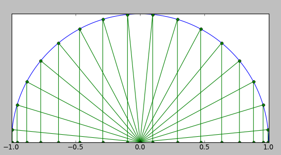
You will note that the nodes are spaced equally near 0 and more compressed towards ± 1.

To approximate a function by a linear combination of the first N Chebyshev polynomials (k=0 to N-1), the coefficient $c_k$ is simply equal to $A\left(k\right)$ times the average of the products $T_k\left(u\right)f\left(x\right)$ evaluated at the N Chebyshev nodes, where $A=1$ for $k=0$ and $A=2$ for all other k.

Let's illustrate the process more clearly with an example.

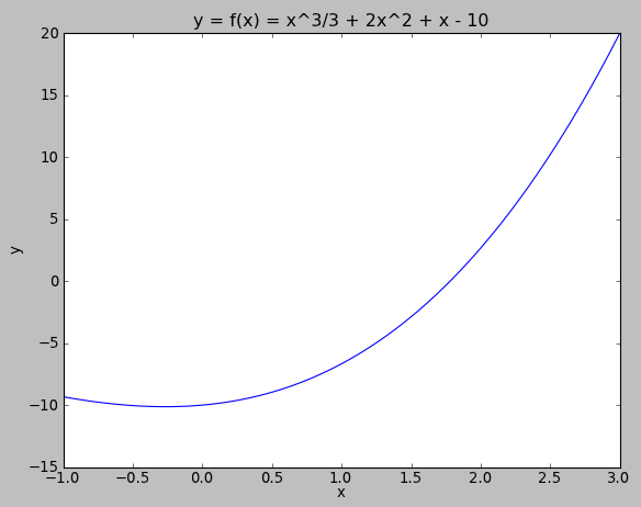
Suppose $f\left(x\right)=\frac{1}{3}{x}^3+2x^2+x-10$ over the range $[-1,3]$, with $u=\frac{x-1}{2},x=2u+1$:

Let's use $N=5$. The Chebyshev nodes for N=5 are $u=-0.951057,-0.587785,0,+0.587785,+0.951057$. This corresponds to $x=-0.902113,-0.175571,1,2.175771,2.902113$, and the function $f\left(x\right)$ evaluated at those nodes are $y=-9.51921,-10.11572,-6.66667,5.07419,17.89408$.

For $c_0$ we compute the average value of y = $(-9.51921-10.11572-6.66667+5.07419+17.89408)/5=-0.66667$.

For $c_1$ we compute 2 × the average value of u × y = $2\times (-9.51921\times -0.951057+-10.11572\times -0.587785$ $+-6.66667\times 0+5.07419\times 0.587785+17.89408\times 0.951057)=14$

For $c_2$ we compute 2 × the average value of $T_2\left(u\right)\times y=(2u^2-1)\times y⟶c_2=6$

For $c_3$ we compute 2 × the average value of $T_3\left(u\right)\times y=(4u^3-3u)\times y⟶c_3=0.66667$

For $c_4$ we compute 2 × the average value of $T_4\left(u\right)\times y=(8u^4-8u^2+1)\times y⟶c_4=0$

The conclusion here is that $f\left(x\right)=-\frac{2}{3}{T}_0\left(u\right)+14T_1\left(u\right)+6T_2\left(u\right)+\frac{2}{3}{T}_3\left(u\right)$ ; if you go and crunch through the algebra you will see that the result is the same as $f\left(x\right)=\frac{1}{3}{x}^3+2x^2+x-10$.

So what was the point here....? Well, if you already have the coefficients of a polynomial, there's no point in using Chebyshev polynomials. (If the input range is significantly different from $[1,1]$, a linear transformation from x to u where $u\in [-1,1]$ will give you a polynomial in u that has better numerical stability, and Chebyshev polynomials are one way to do this transformation. More on this later) If you want to approximate the polynomial with a polynomial of lesser degree, Chebyshev polynomials will give you the best approximation.

For example let's use a quadratic function to approximate $f\left(x\right)$ over the input range in question. All we need to do is truncate the Chebyshev coefficients: let's compute$$\begin{array}{ccc}{f}_2\left(x\right)& =& -\frac{2}{3}{T}_0\left(u\right)+14T_1\left(u\right)+6T_2\left(u\right)\\ & =& -\frac{2}{3}+14u+6\times (2u^2-1)\\ & =& -\frac{20}{3}+14u+12u^2\\ & =& -\frac{20}{3}+7(x-1)+3(x-1{)}^2\\ & =& 3x^2+x-\frac{32}{3}.\end{array}$$

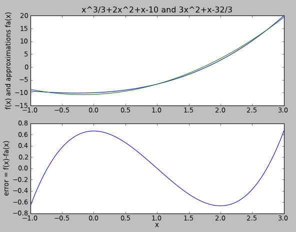
Voila! We have a quadratic function that is close to the original cubic function, and the magnitude of the error is just the coefficient of the Chebyshev polynomial we removed = $\frac{2}{3}$.

You will note that these two polynomials ($\frac{1}{3}{x}^3+2x^2+x-10$ and $3x^2+x-\frac{32}{3}$), expressed in their normal power series form, have no obvious relation to each other, whereas the Chebyshev coefficients are the same except in coefficient $c_3$ which we set to zero to get a quadratic function.

In my view, this is the primary utility of expressing a function in terms of its Chebyshev coefficients: The coefficient $c_0$ tells you the function's average value over the input range; $c_1$ tells you the function's "linearness", $c_2$ tells you the function's "quadraticness", $c_3$ tells you the function's "cubicness", etc.

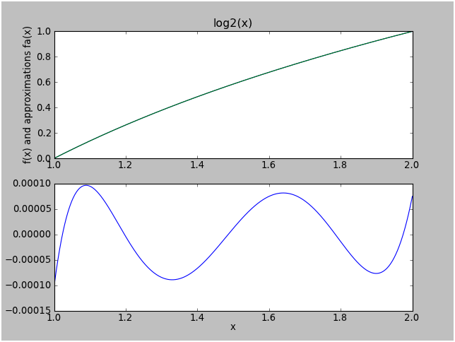
Here's a more typical and less trivial example. Suppose we wish to approximate ${\log }_{2}x$ over the range $[1,2]$.

A decomposition into Chebyshev coefficients up to degree 6 yields the following:

$$\begin{array}{ccc}{c}_0& =& +0.54311\\ c_1& =& +0.49505\\ c_2& =& -0.042469\\ c_3& =& +0.0048577\\ c_4& =& -6.2508\times {10}^{-4}\\ c_5& =& +8.5757\times {10}^{-5}\\ c_6& =& -1.1996\times {10}^{-5}\end{array}$$

You will note that each coefficient is only a fraction of the magnitude of the previous coefficient. This is an indicator that the function in question (over the specified input range) lends itself well to polynomial approximation. If the Chebyshev coefficients don't decrease significantly by the 5th coefficient, I would classify that function as "nonpolynomial" over the range of interest.

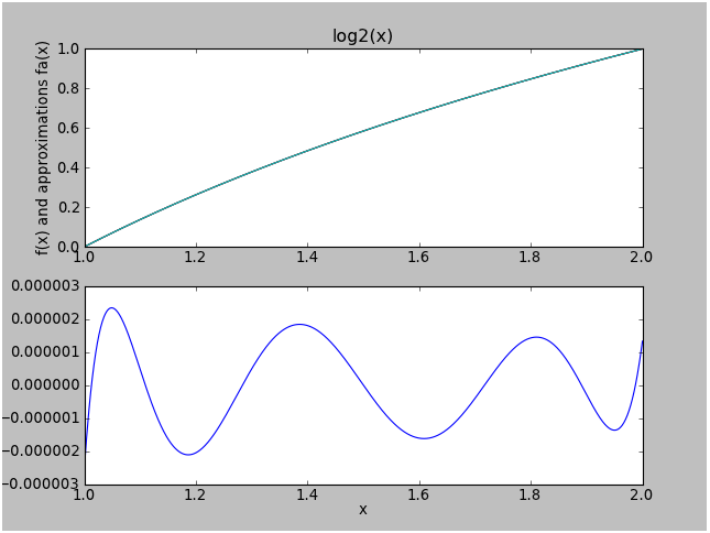
The maximum error for the 6th-degree Chebyshev approximation for ${\log }_{2}x$ over $x\in [1,2]$ is only about 2.2×10-6, which is approximately the value of the next Chebyshev coefficient.

If we truncate the series to a 4th-degree Chebyshev approximation, we get a maximum error that is about equal to $c_5=8.6\times {10}^{-5}$: