https://nextjournal.com/gkoehler/digit-recognition-with-keras

 Micah P. Dombrowski
 Joshua Sierles
 Andrea Amantini
 Philippa Markovics
MNIST Handwritten Digit Recognition in Keras
Gregor Koehler
In this article we'll build a simple neural network and train it on a GPU-enabled server to recognize handwritten digits using the MNIST dataset. Training a classifier on the MNIST dataset is regarded as the hello world of image recognition. To follow along here, you should have a basic understanding of the Multilayer Perceptron class of neural networks.

MNIST contains 70,000 images of handwritten digits: 60,000 for training and 10,000 for testing. The images are grayscale, 28x28 pixels, and centered to reduce preprocessing and get started quicker.
Keras is a high-level neural network API focused on user friendliness, fast prototyping, modularity and extensibility. It works with deep learning frameworks like Tensorflow, Theano and CNTK, so we can get right into building and training a neural network without a lot of fuss.
Let's get started by setting up our environment with Keras using Tensorflow as the backend.
Setting up the Environment
First, we have to install the Tensorflow and Keras packages. We do this in a separate runtime so that we can save it and export as a new environment and never have to install again.
conda install -y -c anaconda \ tensorflow-gpu h5py cudatoolkit=8 pip install kerasWe'll also import the dataset to cache it.
python -c 'from keras.datasets import mnistmnist.load_data()'Preparing the Dataset
These package imports are pretty standard — we'll get back to the Keras-specific imports further down.
nvidia-smi# imports for array-handling and plottingimport numpy as npimport matplotlibmatplotlib.use('agg')import matplotlib.pyplot as plt# let's keep our keras backend tensorflow quietimport osos.environ['TF_CPP_MIN_LOG_LEVEL']='3'# for testing on CPU#os.environ['CUDA_VISIBLE_DEVICES'] = ''# keras imports for the dataset and building our neural networkfrom keras.datasets import mnistfrom keras.models import Sequential, load_modelfrom keras.layers.core import Dense, Dropout, Activationfrom keras.utils import np_utilsNow we'll load the dataset using this handy function which splits the MNIST data into train and test sets.
(X_train, y_train), (X_test, y_test) = mnist.load_data()Let's inspect a few examples. The MNIST dataset contains only grayscale images. For more advanced image datasets, we'll have the three color channels (RGB).
fig = plt.figure()for i in range(9): plt.subplot(3,3,i+1) plt.tight_layout() plt.imshow(X_train[i], cmap='gray', interpolation='none') plt.title("Digit: {}".format(y_train[i])) plt.xticks([]) plt.yticks([])figIn order to train our neural network to classify images we first have to unroll the height
fig = plt.figure()plt.subplot(2,1,1)plt.imshow(X_train[0], cmap='gray', interpolation='none')plt.title("Digit: {}".format(y_train[0]))plt.xticks([])plt.yticks([])plt.subplot(2,1,2)plt.hist(X_train[0].reshape(784))plt.title("Pixel Value Distribution")figAs expected, the pixel values range from 0 to 255: the background majority close to 0, and those close to 255 representing the digit.
Normalizing the input data helps to speed up the training. Also, it reduces the chance of getting stuck in local optima, since we're using stochastic gradient descent to find the optimal weights for the network.
Let's reshape our inputs to a single vector vector and normalize the pixel values to lie between 0 and 1.
# let's print the shape before we reshape and normalizeprint("X_train shape", X_train.shape)print("y_train shape", y_train.shape)print("X_test shape", X_test.shape)print("y_test shape", y_test.shape)# building the input vector from the 28x28 pixelsX_train = X_train.reshape(60000, 784)X_test = X_test.reshape(10000, 784)X_train = X_train.astype('float32')X_test = X_test.astype('float32')# normalizing the data to help with the trainingX_train /= 255X_test /= 255# print the final input shape ready for trainingprint("Train matrix shape", X_train.shape)print("Test matrix shape", X_test.shape)So far the truth (Y in machine learning lingo) we'll use for training still holds integer values from 0 to 9.
print(np.unique(y_train, return_counts=True))Let's encode our categories - digits from 0 to 9 - using one-hot encoding. The result is a vector with a length equal to the number of categories. The vector is all zeroes except in the position for the respective category. Thus a '5' will be represented by [0,0,0,0,1,0,0,0,0].
# one-hot encoding using keras' numpy-related utilitiesn_classes = 10print("Shape before one-hot encoding: ", y_train.shape)Y_train = np_utils.to_categorical(y_train, n_classes)Y_test = np_utils.to_categorical(y_test, n_classes)print("Shape after one-hot encoding: ", Y_train.shape)Building the Network
Let's turn to Keras to build a neural network.
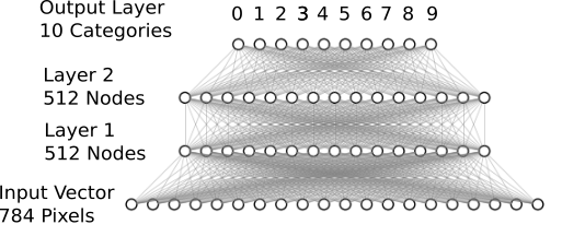
Our densely-connected network with two hidden layers.
Our pixel vector serves as the input. Then, two hidden 512-node layers, with enough model complexity for recognizing digits. For the multi-class classification we add another densely-connected (or fully-connected) layer for the 10 different output classes. For this network architecture we can use the Keras Sequential Model. We can stack layers using the .add() method.
When adding the first layer in the Sequential Model we need to specify the input shape so Keras can create the appropriate matrices. For all remaining layers the shape is inferred automatically.
In order to introduce nonlinearities into the network and elevate it beyond the capabilities of a simple perceptron we also add activation functions to the hidden layers. The differentiation for the training via backpropagation is happening behind the scenes without having to implement the details.
We also add dropout as a way to prevent overfitting. Here we randomly keep some network weights fixed when we would normally update them so that the network doesn't rely too much on very few nodes.
The last layer consists of connections for our 10 classes and the softmax activation which is standard for multi-class targets.
# building a linear stack of layers with the sequential modelmodel = Sequential()model.add(Dense(512, input_shape=(784,)))model.add(Activation('relu')) model.add(Dropout(0.2))model.add(Dense(512))model.add(Activation('relu'))model.add(Dropout(0.2))model.add(Dense(10))model.add(Activation('softmax')) Interested in a new type of notebook?
Try Nextjournal. The notebook for reproducible research.
- Automatically version-controlled all the time
- Supports Python, R, Julia, Clojure and more
- Invite co-workers, collaborate in real-time
- Import your existing Jupyter notebooks
Compiling and Training the Model
Now that the model is in place we configure the learning process using .compile(). Here we specify our loss function (or objective function). For our setting categorical cross entropy fits the bill, but in general other loss functions are available.
As for the optimizer of choice we'll use Adam with default settings. We could also instantiate an optimizer and set parameters before passing it to model.compile() but for this example the defaults will do.
We also choose which metrics will be evaluated during training and testing. We can pass any list of metrics - even build metrics ourselves - and have them displayed during training/testing. We'll stick to accuracy for now.
# compiling the sequential modelmodel.compile(loss='categorical_crossentropy', metrics=['accuracy'], optimizer='adam')Having compiled our model we can now start the training process. We have to specify how many times we want to iterate on the whole training set (epochs) and how many samples we use for one update to the model's weights (batch size). Generally the bigger the batch, the more stable our stochastic gradient descent updates will be. But beware of GPU memory limitations! We're going for a batch size of 128 and 8 epochs.
To get a handle on our training progress we also graph the learning curve for our model looking at the loss and accuracy.
In order to work with the trained model and evaluate its performance we're saving the model in /results/.
# training the model and saving metrics in historyhistory = model.fit(X_train, Y_train, batch_size=128, epochs=20, verbose=2, validation_data=(X_test, Y_test))# saving the modelsave_dir = "/results/"model_name = 'keras_mnist.h5'model_path = os.path.join(save_dir, model_name)model.save(model_path)print('Saved trained model at %s ' % model_path)# plotting the metricsfig = plt.figure()plt.subplot(2,1,1)plt.plot(history.history['acc'])plt.plot(history.history['val_acc'])plt.title('model accuracy')plt.ylabel('accuracy')plt.xlabel('epoch')plt.legend(['train', 'test'], loc='lower right')plt.subplot(2,1,2)plt.plot(history.history['loss'])plt.plot(history.history['val_loss'])plt.title('model loss')plt.ylabel('loss')plt.xlabel('epoch')plt.legend(['train', 'test'], loc='upper right')plt.tight_layout()figThis learning curve looks quite good! We see that the loss on the training set is decreasing rapidly for the first two epochs. This shows the network is learning to classify the digits pretty fast. For the test set the loss does not decrease as fast but stays roughly within the same range as the training loss. This means our model generalizes well to unseen data.
Evaluate the Model's Performance
It's time to reap the fruits of our neural network training. Let's see how well we the model performs on the test set. The model.evaluate() method computes the loss and any metric defined when compiling the model. So in our case the accuracy is computed on the 10,000 testing examples using the network weights given by the saved model.
mnist_model = load_model(keras_mnist.h5)loss_and_metrics = mnist_model.evaluate(X_test, Y_test, verbose=2)print("Test Loss", loss_and_metrics[0])print("Test Accuracy", loss_and_metrics[1])This accuracy looks very good! But let's stay neutral here and evaluate both correctly and incorrectly classified examples. We'll look at 9 examples each.
# load the model and create predictions on the test setmnist_model = load_model(keras_mnist.h5)predicted_classes = mnist_model.predict_classes(X_test)# see which we predicted correctly and which notcorrect_indices = np.nonzero(predicted_classes == y_test)[0]incorrect_indices = np.nonzero(predicted_classes != y_test)[0]print()print(len(correct_indices)," classified correctly")print(len(incorrect_indices)," classified incorrectly")# adapt figure size to accomodate 18 subplotsplt.rcParams['figure.figsize'] = (7,14)figure_evaluation = plt.figure()# plot 9 correct predictionsfor i, correct in enumerate(correct_indices[:9]): plt.subplot(6,3,i+1) plt.imshow(X_test[correct].reshape(28,28), cmap='gray', interpolation='none') plt.title( "Predicted: {}, Truth: {}".format(predicted_classes[correct], y_test[correct])) plt.xticks([]) plt.yticks([])# plot 9 incorrect predictionsfor i, incorrect in enumerate(incorrect_indices[:9]): plt.subplot(6,3,i+10) plt.imshow(X_test[incorrect].reshape(28,28), cmap='gray', interpolation='none') plt.title( "Predicted {}, Truth: {}".format(predicted_classes[incorrect], y_test[incorrect])) plt.xticks([]) plt.yticks([])figure_evaluationAs we can see, the wrong predictions are quite forgiveable since they're in some cases even hard to recognize for the human reader.
In summary we used Keras with a Tensorflow backend on a GPU-enabled server to train a neural network to recognize handwritten digits in under 20 seconds of training time - all that without having to spin up any compute instances, only using our browser.
In the next article of this series (coming soon) we'll harness the power of GPUs even more to train more complex neural networks which include convolutional layers.
Interested in a new type of notebook?Try Nextjournal. The notebook for reproducible research.
- Automatically version-controlled all the time
- Supports Python, R, Julia, Clojure and more
- Invite co-workers, collaborate in real-time
- Import your existing Jupyter notebooks
No hay comentarios:
Publicar un comentario