Chebyshev polynomials and interpolation

https://drlvk.github.io/nm/section-chebyshev-polynomials-interpolation.html

Chebyshev polynomials and interpolation

22.2 Chebyshev polynomials and interpolation

🔗

In Chapter 15 we studied Legendre polynomials $P_n$ which are orthogonal on the interval $[-1,1]$ in the sense that ${\int }_{-1}^1{P}_n\left(x\right)P_k\left(x\right)dx=0$ when $n\ne k\text{.}$ We also use Laguerre polynomials $L_n$ which are orthogonal on $[0,\infty )$ with the weight function $e^{-x}\text{,}$ meaning that ${\int }_{-1}^1{L}_n\left(x\right)L_k\left(x\right)e^{-x}dx=0$ when $n\ne k\text{.}$ The Chebyshev polynomials $T_n$ are orthogonal on the interval $[-1,1]$ with the weight function $1/\sqrt{1-x^2}\text{,}$ meaning that

$${\int }_{-1}^1{T}_n\left(x\right)T_k\left(x\right)\frac{dx}{\sqrt{1-x^2}}=0\text{when}n\ne k$$

🔗

As for other families of orthogonal polynomials, we have a recursive formula for Chebyshev polynomials: starting with $T_0\left(x\right)=1$ and $T_1\left(x\right)=x$ we can compute the rest as

$$\begin{array}{}{T}_{n+1}\left(x\right)=2x{T}_n\left(x\right)-T_{n-1}\left(x\right)& \text{(22.2.1)}\end{array}$$

🔗

The recursion is simpler than for $P_n$ or $L_n\text{:}$ there is no division, so all polynomials $T_n$ have integer coefficients.

🔗

Example 22.2.1. Plot Chebyshev polynomials $T_n$. 

🔗

Example 22.2.1 indicates that Chebyshev polynomials oscillate between $-1$ and $1$ on the interval $[-1,1]\text{.}$ The following remarkable identity confirms this observation:

Example 22.2.1. Plot Chebyshev polynomials $T_n$. 

 

Recursively find the coefficients of Chebyshev polynomials $T_n$ for $n\le 6\text{.}$ Plot all of them on the interval $[-1,1]\text{.}$

Answer

This is a straightforward modification of Example 15.4.1.

p = [1];
q = [1 0];
x = linspace(-1, 1, 1000);
hold on
plot(x, polyval(p, x), x, polyval(q, x));

for n = 1:5
    r = 2*[q 0] - [0 0 p];
    p = q;
    q = r;
    plot(x, polyval(r, x))
end
hold off

in-context

$$\begin{array}{}{T}_n\left(\cos \theta \right)=\cos \left(n\theta \right)& \text{(22.2.2)}\end{array}$$

🔗

for all $\theta \in R\text{.}$ The proof is by induction. Base of induction is $n=0,1\text{:}$ for $T_0\left(x\right)=1$ and $T_1\left(x\right)=x$ the validity of (22.2.2) is obvious. For the inductive step, assume (22.2.2) holds for $T_0,\dots ,T_n$ and use (22.2.1):

$$\begin{array}{}{T}_n\left(\cos \theta \right)=\cos \left(n\theta \right)& \text{(22.2.2)}\end{array}$$

in-context

$$T_{n+1}\left(\cos \theta \right)=2\cos \theta \cos \left(n\theta \right)-\cos \left(\right(n-1\left)\theta \right)=\cos \left(\right(n+1\left)\theta \right)$$

🔗

where the second step involves the identity

$$2\cos \alpha \cos \beta =\cos (\alpha -\beta )+\cos (\alpha +\beta )$$

🔗

The right hand side of (22.2.2) is zero when $n\theta$ is an odd multiple of $\pi /2\text{,}$ hence $\theta =(2k-1)\frac{\pi }{2n}\text{.}$ Plugging $k=1,\dots ,n$ we find that

$$\begin{array}{}{T}_n\left(\cos \theta \right)=\cos \left(n\theta \right)& \text{(22.2.2)}\end{array}$$

in-context

$$\begin{array}{}{T}_n\left(x\right)=0\text{when}x=\cos \left(\right(2k-1\left)\frac{\pi }{2n}\right),k=1,\dots ,n& \text{(22.2.3)}\end{array}$$

🔗

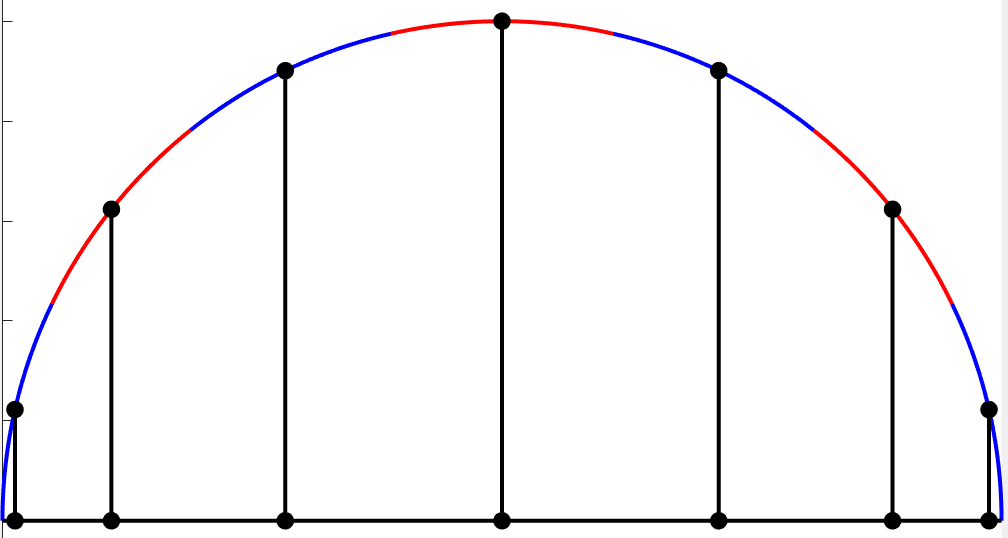
and since the polynomial $T_n$ can have at most $n$ real roots, these are all of its roots. They are easy to visualize: draw a semi-circle with interval $[a,b]$ as diameter, divide it into $n$ equal arcs, and project the midpoint of each arc back to the interval.

🔗

Figure 22.2.2. Chebyshev points of the first kind

🔗

The recursive formula shows that the leading coefficient of $T_n$ is $2^{n-1}\text{.}$ Therefore,

$$T_n\left(x\right)=2^{n-1}\prod _{k=1}^n(x-x_k)$$

🔗

where $x_1,\dots ,x_n$ are the roots (22.2.3). It follows that the absolute value of the product ${\prod }_{k=1}^n(x-x_k)$ is bounded by $2^{1-n}\text{.}$ It can be proved that $2^{1-n}$ is as small as one can get for any choice of $n$ points on the interval $[-1,1]\text{.}$ This suggests that Chebyshev points should work well for polynomial interpolation, and they do. Let us re-do Example 21.2.2 with random data to illustrate this.

Example 21.2.2. Plot the Lagrange polynomial through 10 points. 

 

Plot the Lagrange polynomial each of the following data sets:

1. the points $(k,\sin k)\text{,}$ $k=1,\dots ,10\text{;}$
2. the points with $x_k$ as above, and $y_k$ chosen randomly from the standard normal distribution.

Answer

n = 10;
x = 1:n;
y = sin(x);  % or y = randn(1, n);
w = ones(1, n);
for k = 1:n
    for j = 1:n
        if j ~= k
            w(k) = w(k)/(x(k)-x(j));
        end
    end
end

p = @(t) (y.*w*(t - x').^(-1)) ./ (w*(t - x').^(-1));
t = linspace(min(x)-0.01, max(x)+0.01, 1000);
plot(t, p(t), x, y, 'r*')

The double loop computes the weights w which do not involve the argument of the interpolating polynomial p. This argument is called t because x is already used for the data points. The interval for plotting is chosen to contain the given x-values with a small margin on both sides: this helps both visualization and evaluation, because we avoid plugging in $t=x_1,x_n\text{.}$ The barycentric evaluation of the polynomial is vectorized. When t is a scalar, t - x' is a column vector. Taking reciprocals element-wise gives another column vector. Dot-product with w or y.*w implements the sums such as ${\sum }_{k=1}^n{w}_k/(t-x_k)\text{.}$

How does p accept a row vector as t? The expression t - x' is the difference of a row vector and a column vector; in Matlab this creates a matrix where $(i,j)$ entry is $t_j-x_i\text{.}$ Subsequent operations proceed as above, and the result is a row vector of values $p\left(t\right)\text{.}$

in-context

$$\begin{array}{}{T}_n\left(x\right)=0\text{when}x=\cos \left(\right(2k-1\left)\frac{\pi }{2n}\right),k=1,\dots ,n& \text{(22.2.3)}\end{array}$$

in-context

🔗

Example 22.2.3. An interpolating polynomial using Chebyshev points. 

🔗

Running the code Example 22.2.3 several times, we see that the interpolating polynomial behaves reasonably, without unnatural oscillations that come from interpolating at equally spaced points.

Example 22.2.3. An interpolating polynomial using Chebyshev points. 

 

Let $x_1,\dots ,x_{10}$ be the roots of $T_{10}\text{.}$ Choose $y_k$ randomly from the standard normal distribution, and draw the interpolating polynomial through the points $(x_k,y_k)\text{.}$

Answer

The only change to Example 21.2.2 is replacing the x-coordinates.

n = 10;
x = cos((2*(1:n)-1)*pi/(2*n)); 
y = randn(1, n);
w = ones(1, n);
for k = 1:n
    for j = 1:n
        if j ~= k
            w(k) = w(k)/(x(k)-x(j));
        end
    end
end

p = @(t) (y.*w*(t - x').^(-1)) ./ (w*(t - x').^(-1));
t = linspace(min(x)-0.01, max(x)+0.01, 1000);
plot(t, p(t), x, y, 'r*')