http://www.katjaas.nl/fourier/fourier.html
Fourier Matrix
Imagine you have a signal and you want to examine how much of a certain frequency is in that signal. That could be done with two convolutions. The signal would be convolved with the two orthogonal phases, sine and cosine, of the frequency under examination. At every samplemoment two inner products will tell the (not yet normalised) correlation over the past N samples. Below, I plotted an example of sine and cosine vectors doing one cycle in N = 8 samples:
 |
Recall that convolution vectors always appear time-reversed in the convolution matrix. To time-reverse a sine-cosine set we do not need to inspect the signal sample by sample to flip the array. Take a look at the plot below, and the next one. A set of cosine and negative sine has exactly the same property as a time-reversed set.
 |
In complex number terminology, it is the complex conjugate. cos(x)+isin(x) becomes cos(x)-isin(x):
 |
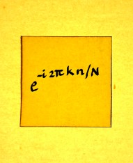
These vectors can be described as an array of complex numbers cos(2*pi*n/8)-isin(2*pi*n/8) or as complex exponentials e-i2*pi*n/8. The complex numbers or exponentials are on the unit circle in the complex plane, with the series showing a negative (=clockwise, yes) rotation:
 |
To compute these convolutions would require 2 times 8 multiplications, is 16 multiplications per samplemoment, and almost as many additions. Now imagine you would like to detect more frequencies than only this one. For lower frequencies the arrays must be longer. At a typical samplerate of 44.1 KHz, one period of 40Hz stretches over more than a thousand samples.
Computing convolutions with thousand-or-more-point arrays, just to find a frequency in a signal, would be a ludicrous waste of computational effort. After all, the amplitude in a complex sinusoid vector is perfectly constant. Therefore it would almost suffice to take a snapshot of the signal every N moments, and compute the inner product once over that period. This will come at the price of probable jumps at the boundaries of the snapshot. Such jumps form artefacts which will distort the correlation. So the snapshot method is a compromise. But a necessary one, specially since you may want to detect more frequencies, covering the whole spectrum.
Convolution with 'snapshots' is not convolution in the proper sense. Though it can be filed under 'block-convolution'. With block-convolution, we could resolve up to N frequencies (conjugates or aliases included) in each N-point snapshot. The block of a Discrete Fourier Transform is an NxN square matrix with complex entries. The blocks themselves are positioned on the main diagonal of a bigger matrix. We will take a look at that from a bird's-eye-perspective:
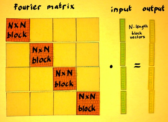 |
Compared to regular convolution, a big difference is: the shift in the rows of the Fourier matrix. It shifts rightwards with N samples at a time instead of one sample at a time. It also shifts downwards with N samples at a time. The output is therefore no longer one signal, but N interleaved points of N separate N-times downsampled signals. Which were filtered by the N different vectors in the Fourier block.
This is not a conventional interpretation of Discrete Fourier Transform. But I do not worry about that. There is enough conventional descriptions of Fourier Transform in textbooks and on the web.
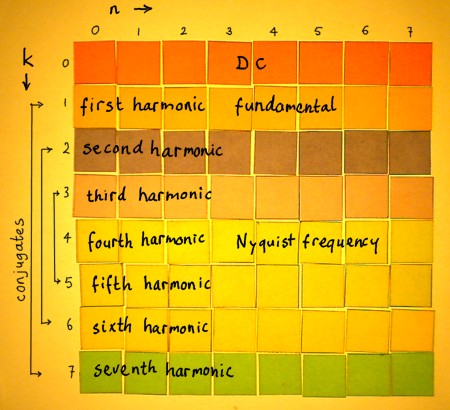
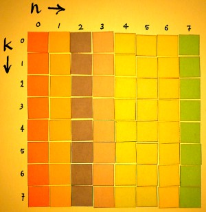
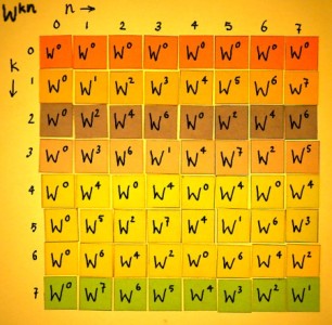
Let us now find out how to fill a Fourier block. Our example is with N=8. We need to construct 8 complex vectors of different (orthogonal) frequencies. Because I have the habit of indexing signals with n, like x[n], I will reserve index k for the frequencies. The frequencies go in the rows of the matrix.
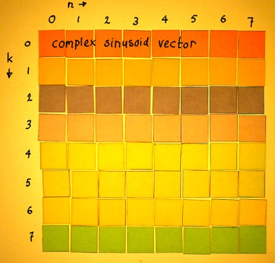 |
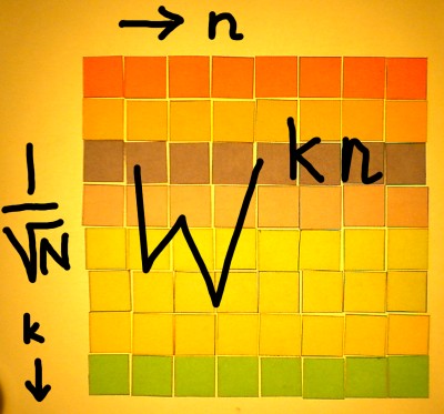
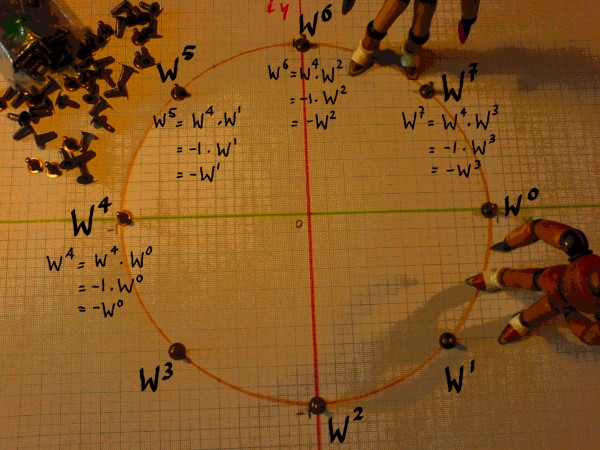
All entries will be filled with complex exponentials e-i2*pi*k*n/N. For convenience, we write e-i2*pi*k*n/N = Wk*n. Then, the Fourier matrix can be simply denoted: the Wk*n matrix. No matter how big it is. There is always just as many frequencies k as there are sample values n.
 |
In this definition, W can be recognised as a complex number constant, defined by the value of N. The number N divides the unit circle in N equal portions. W is the first point in clockwise direction, thereby establishing the basic angular interval of the matrix.
 |
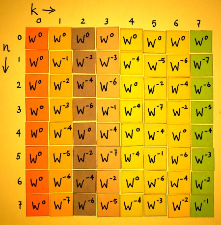
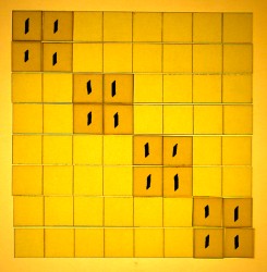
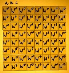
In the figure below, the matrix is filled with the Wkn powers:
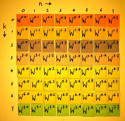 |
Do the multiplications:
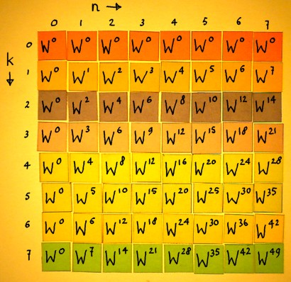 |
Row number k=0 represents DC, with e-i2*pi*k*n/N being e0i in every entry. Row number k=1 represents the fundamental frequency of the matrix, doing one cycle in 8 samples. This is the complex vector that I took as the first example earlier on this page. Row number k=2 represents a frequency going twice as fast. It is the second harmonic. Here is a plot of sine and cosine in the second harmonic:
 |
The third harmonic does three cycles in 8 samples:
 |
Everytime, complex exponentials of the fundamental period are recycled. No new exponentials will appear. Here is how the third harmonic moves round the unit circle on the complex plane:
 |
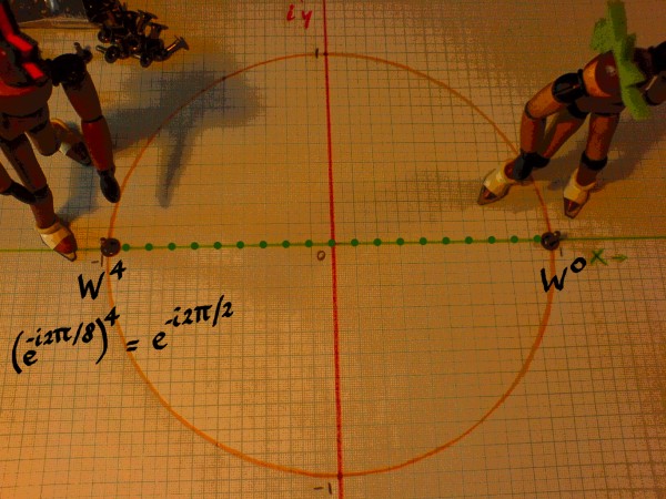
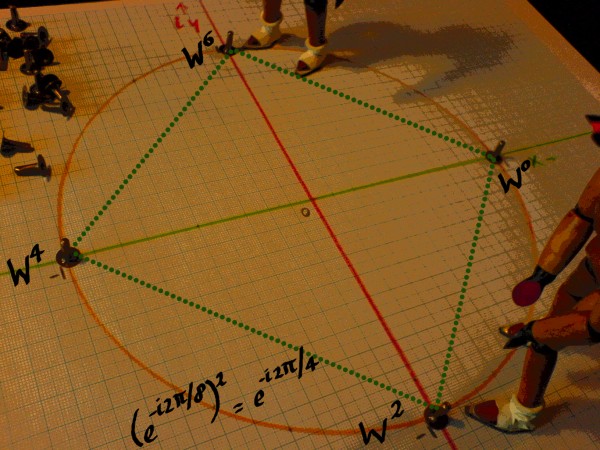
The next one is the fourth harmonic. In the case of N=8, the fourth harmonic is the famous Nyquist-frequency. Sine cannot exist here. On the complex plane, the only points are -1 and 1 on the x-axis.
 |
The fifth harmonic is the mirror-symmetric version of the third harmonic.
 |
When their iterations over the unit circle are compared, their kinship is clear:
 |
 |
They are conjugates. To put it in other words: if the third harmonic would rotate in reversed direction, it would be identical to the fifth harmonic. But all harmonics have a well-defined rotational direction, because they are complex. All vectors are unique, and orthogonal to each other. Such conjugate distinction, by the way, can not exist in a real (input) signal: there we speak of aliases.
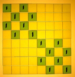
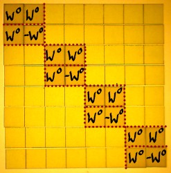
The sixth and seventh harmonic are also conjugates of other harmonics in the matrix. When an overview of the harmonics is made, it becomes clear that row k=0 and row k=4 have no conjugates. These are DC and Nyquist-frequency.
 |
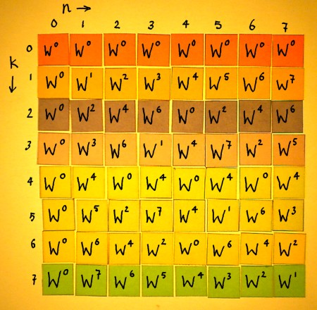
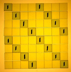
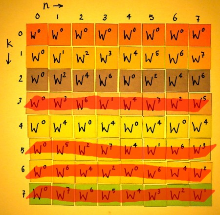
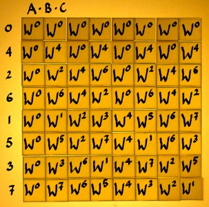
Because the powers Wkn are periodic modulo N, the vectors can be rewritten. W8 is equal to W0, W9 is W1 etcetera. It is integer division by 8, and the remainder is the new exponent of W. In the rewritten Fourier matrix for N=8, the conjugates display themselves quite clearly:
 |
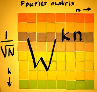
We are not completely done with the Fourier matrix yet, because it needs normalisation. There is a certain freedom, to choose a normalisation type according to the purpose of the transform. I have done a separate page on that because it is too complicated to describe in just a few words. But strictly speaking, a normalised vector is a vector with norm 1, or unity total amplitude. That requires a normalisation factor 1/N1/2 for all entries of the Wkn matrix. In that case, the Fourier matrix is orthonormal, and the transpose of it is exactly the inverse. An orthonormal Fourier matrix can be defined:
 |
The output of the matrix operation is called 'spectrum'. It expresses the input content in terms of the trigonometric functions of the Fourier matrix. These functions are pure rotations, and the output coefficients tell the amount of each, as found in the input. The normalisation type is crucial to the interpretation of these coefficients. And the transform block-width N is decisive for the frequency resolution.
Apart from being informative about frequencies, the coefficients have other virtues. They can be exploited to manipulate the frequency content. After such manipulation, the inverse Fourier Transform can revert the spectrum back to where it came from: time, space, or whatever the input represented.
To construct the inverse Fourier matrix, we have to find the transpose. Normally, that can be done by turning the rows into columns. So it would look something like this:
 |
But I have not yet written the entries, because there is something special with these. They are complex, and need to be transposed as well. This is a good moment to inspect the complex entries in detail. On the matrix pages I described complex multiplication more than once. It has a 2x2 square matrix. Therefore, one complex Wkn entry is actually four real entries:
 |
 |
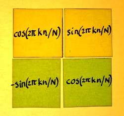 |
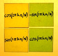
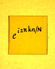
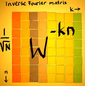
When the rows of the 2x2 matrix become the columns, we simply get the complex conjugate. The complex exponential then rotates anti-clockwise, which is called positive. The sign in the exponent of Wkn must flip and it becomes W-kn.
 |
 |
 |
Now I can write the Wkn powers in the entries of the transpose:
 |
The only difference with the original matrix is the direction of rotation. Apart from their sign, the powers of W have not changed. The matrix is almost symmetric over it's diagonal. The only thing that is not symmetric, is hidden within the 2x2 complex matrices behind the Wkn entries.
The normalised Fourier matrix and it's inverse can be visualised:
 |
 |
It can be written algebraically, with the hatted x being the transformed array:
 |
And the inverse transform:
 |
Discrete Fourier Transform is a very clear and systematic operation, therefore the description of it can be so concise. But the formula is only the principle of DFT. Implementation of the transform will require adaptations, in order to reduce the amount of computations in one way or another. For the transform of a real signal with small block-width N, computation of the conjugates can be skipped. For large N, factorisation of the complex matrix makes for efficient algorithms. Then we speak of the Fast Fourier Transform. Whish I could sketch an FFT operation with my coloured square paperlets....
Fast Fourier Transform
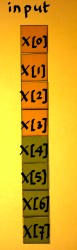
On this page I want to figure out a modest example of Fast Fourier Transform. Even for the simplest form of FFT, we need quite some ingredients:
- a standard complex Discrete Fourier Transform matrix, like it is pictured on the previous page Fourier Matrix
- a generic recipe for matrix decomposition, as sketched on the page Sparse Matrices
- roots of unity, roots of roots, roots of roots of roots, as described on the page Roots of Unity
- a method for phase decomposition / interleaving, as explored on
the page Phase
Decomposition
 |
 |
We are going to decompose the Fourier matrix into three sparse matrices of the form that was sketched earlier. Recall that these were aggregates of identity matrices at different resolutions. On the left is an aggregate of 16 1x1 identity matrices, in the middle we have eight 2x2 identities, and the right matrix is composed of four 4x4 identities. All these identities must be replaced by Wkn powers. Somehow.
 |
 |
 |
Well for the moment it is better to think in terms of roots instead of powers. My page Roots of Unity demonstrated how a whole set of Fourier harmonics can be generated while multiplying and adding merely the 'octaves', which are related to each other as squares and square roots. This is a phenomenon that we can use for the matrix decomposition.
The square roots of unity have W0 and W4 in the N=8 case, as is shown in the picture below:
 |
The square root of the square root is the fourth root. Expressed as powers of W=e-i2pi/8, the fourth roots of one are: W0, W2, W4 and W6.
 |
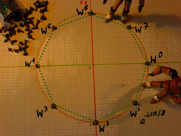
Taking the square root of the fourth root we land at the 8th root finally. For N=8, we can not go further than this.
 |
On the Fourier Matrix page the sine and cosine series for these cases were plotted. I put those plots together here:
 |
Samples of the square roots of unity |
 |
Samples of the fourth-roots of unity |
 |
Samples of the eight-roots of unity |
There is still one important series missing. It is the first root of unity, or 11/1, and it's powers.
 |
That sounds quite trivial indeed. But the fact that W0 operates as an identity follows from our definition of W as being a complex root of unity. I feel we should remain aware of that. W0 is the most-present root in the Fourier matrix. It's power series dominates the FFT. The series forms an identity with respect to rotation. It is a conservator of frequencies.
 |
Samples of the first-root of unity |
Let us look at the Wkn matrix once more, and confirm which harmonics we are going to use, and which ones are skipped:
 |
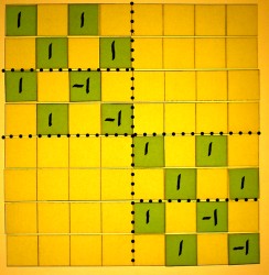
The question is now, how are we to arrange these frequencies in our N=8 sparse factor matrices? Sure this can be derived from the DFT formula, using a sequence of equations. These are fairly complicated however, and I always lose track at some point when studying them. Otherwise, there are these butterfly schemes that accompany most texts on FFT. But I am not a fan of that either. Maybe it is an idea to translate an FFT butterfly scheme to a matrix representation.
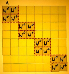
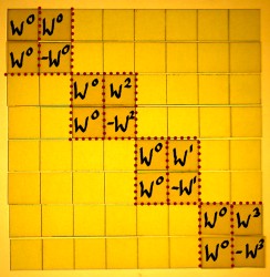
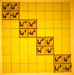
To find a suitable scheme I studied more butterflies than I ever wanted to see, none of them being precisely what I needed. I sort of distilled a form that will serve the purpose of this demonstration. Here we start with the first sparse factor, containing first roots of unity in the upper part and eight-roots of unity in the lower part:
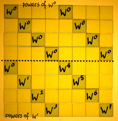 |
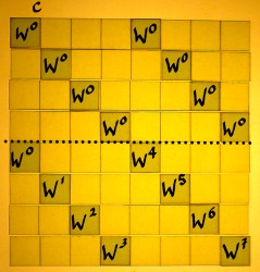
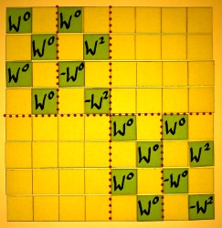
When we consider the next sparse factor as a repetition of the process at another resolution, then we see the W0 series on top again. Powers of W2 are in the lower halves. W0, W2, W4 and W6 are the fourth-roots of unity here.
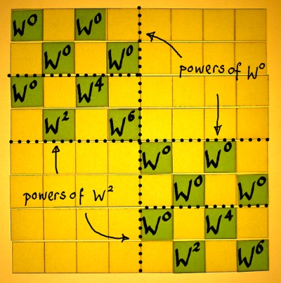 |
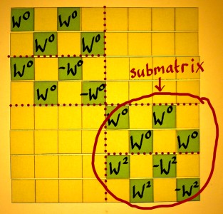
And here is the third sparse factor, it is the last one for the N=8 case. We find the W0 and W4, square roots of unity, in the lower parts of the small submatrices.
 |
For convenience, the three factors are pictured together here:
 |
 |
 |
From these matrices, you could already have the impression that it will split output results into smaller and smaller vectors in every stage. The upper half of each submatrix has merely identities summed, while he lower half has rotations.
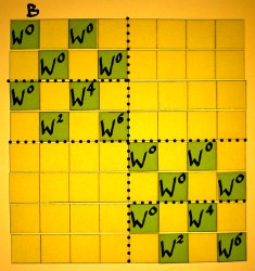
Let us now verify whether these sparse matrices multiplied will really render the complete Wkn matrix. First multiply B with C to get BC.
|
|
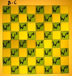 |
Then multiply A with BC to get the full matrix ABC:
|
|
 |
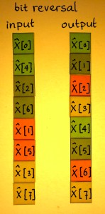
Some of the entries have exponents above 7, and these are to be computed modulo 8. Below we have ABC in a form which can be compared with the Wkn matrix. Hey, it is interesting: all harmonics are present in ABC, but they appear in the wrong order. Actually, they appear in so-called bitreversed order.
 |
 |
If you would use the sketched FFT factors for correlation, the spectrum would appear in decimated or downsampled form. The decimation is an inherent aspect of this FFT process. It happens stepwise: a factor 2 downsampling in each stage. The most efficient solution is to just let it happen. At the end of the process, it can be compensated with a bit-reversed permutation operation, if needed.
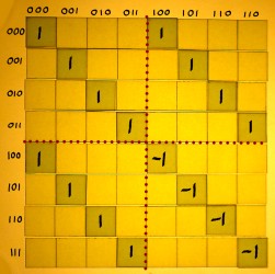
Bit-reversed permutation does in one operation what even-odd decomposition does in several stages. By the way, total decomposition, total interleave, and bit-reversed permutation all have the same effect. A bit-reversed permutation operation is illustrated here, with the indexes of the matrix written as binary numbers:
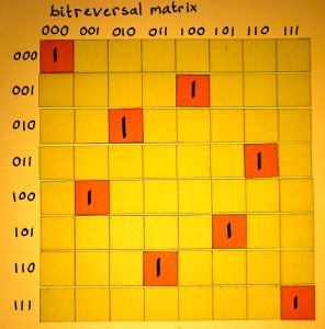 |
 |
The Fast Fourier Transform as sketched on this page can easily be expanded to larger N, if only N is a power of two. It is a radix 2 FFT. Radix means base of the numeral system, and it is the Latin word for root. Radix 2 is only one of the many options for FFT, and even for radix 2, different schemes are possible. I am not going to discuss these alternatives yet, because we are not even ready with our simple example. It can be further decomposed, increasing efficiency one more time. That is for the next page.
Step Two FFT
The previous page showed how a Fourier matrix can be decomposed into sparse factors, making for Fast Fourier Transform. The factor matrices multiplied showed a Fourier Matrix with it's spectrum decimated. For the purpose of that demonstration, the factor matrices were not yet optimally decomposed. On this page we go one step further. Well actually we will go back to our roots once more, the roots of unity.
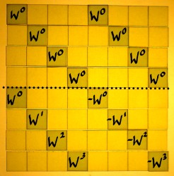
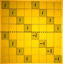
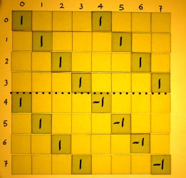
We will make use of this 'identity':
 |
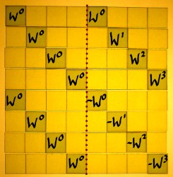
In our N=8 example FFT, WN/2 is W4. For other N it would not be W4 of course. Anyway, -1 is the primitive square root of unity. With the help of this we are going to find aliases that will enable a further reduction in the amount of computations. In the picture below, aliases for W4 till W7 are written down.
 |
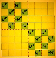
The eight-powers of unity in our FFT matrix are rewritten in this fashion. On the left is the original matrix, the translated version is on the right:
|
 |
Translating the next factor matrix:
|
 |
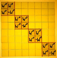
And the last one:
|
 |
So what is our gain here? Normally, you first multiply corresponding cells in vectors and then sum the results to find the inner product. In the radix 2 FFT there is two non-zero entries per row. That would mean two multiplications every time, followed by an addition. But in the case that two multiplication factors were the same, you could first do the addition and then the multiplication. In the above case, the factors are not equal, but almost: only their sign is different. Then it would suffice to first subtract and subsequently multiply. That saves one complex multiplication. Compare with a real number example like: 4*5-2*5=(4-2)*5.
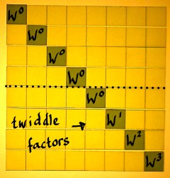
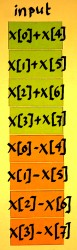
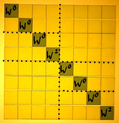
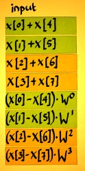
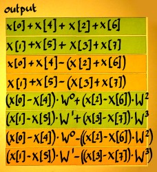
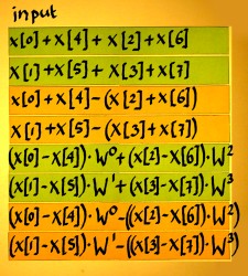
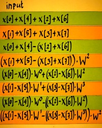
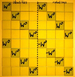
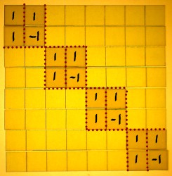
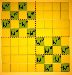
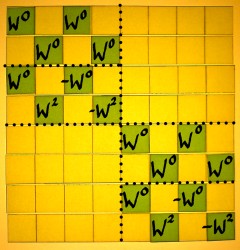
Let me split the first FFT factor into an addition/subtraction part and a rotation part. The rotation matrix has what they call the 'twiddle factors'. The addition/subtraction part comes first, because we work from right to left.
 |
 |
 |
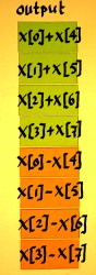
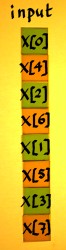
Below, the output of the first matrix operation is illustrated. Subtraction is computationally no more intensive than addition. But in the process, the entries x[4], x[5], x[6] and x[7] get a 'free' rotation by pi radians or half a cycle.
 |
|
 |
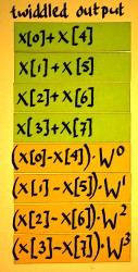
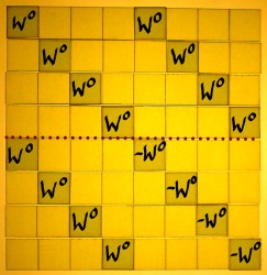
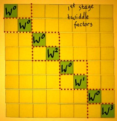
Next comes the multiplication with twiddle factors:
|
 |
 |
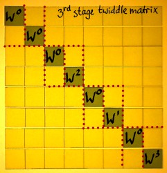
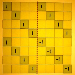
The two remaining FFT stages are decomposed similarly, into an addition/subtraction matrix and a diagonal rotation or 'twiddle' matrix. I will draw these decompositions as well. Here is the second stage as decomposed in addition/subtraction and twiddle matrix:
 |
 |
First do the additions and subtractions. Notice how input and output vectors are treated here as if they were two-point vectors, while in the preceding stage they were four-point vectors.
|
 |
 |
Next comes the twiddle matrix of the second stage:
|
 |
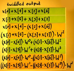 |
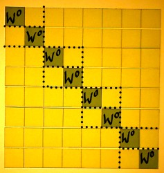
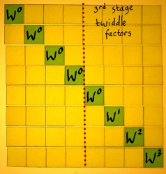
In the third stage, the twiddle matrix has merely W0 factors. This will function as an identity matrix so we do not have to implement it. Only the matrix with additions and subtractions remains to be done.
 |
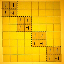 |
The last operation is thus addition and subtraction:
|
 |
 |
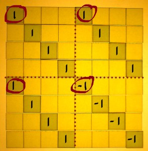
Below, I reorganised the output bins to bitreversed sequence, to have them in their harmonic order. Now you could check if the FFT tricks have worked. Bin number 4 for example, has the even x[n] with positive sign and the odd x[n] with negative sign. This is equivalent to x[0]*W0, x[1]*W4, x[2]*W0, x[3]*W4 etcetera.
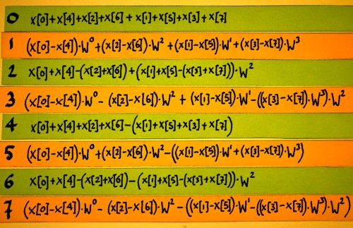 |
The other harmonics require more effort to recognize them as being complex power series. But they all are, it is just that they are computed via another route.
FFT Radix 2 Forms
Even when we confine ourselves to radix 2 FFT, there are four basic schemes. They are the classic Cooley-Tukey and Sande-Tukey algorithms. Only one of these was illustrated on the preceding pages. I want to explore the other three schemes as well. They have so much in common, yet the differences are decisive and they are not to be mixed or confused. First I will discuss some details of these differences. At the end of this page, the four schemes are put together, for overview. They are matrix visualisations of butterfly graphs like those printed in The Fast Fourier Transform (p. 181) by E. Orhan Brigham.
For comparison, here is the scheme as it was illustrated on the previous page:
|
|
|
|
The second scheme differs from the first one in the sense that it starts with the square roots of unity, instead of ending with them. Recall that we work from right to left. Further, the identity parts and rotation parts are now left/right organised, instead of top/bottom. The output of this scheme would have a decimated spectrum as well.
 |
 |
 |
|
Using this scheme, the twiddle matrix would precede the additions and subtractions, in every stage. As an example I will decompose the third stage:
 |
 |
 |
The twiddle factors do not appear in their natural order. From my small example it is hard to see the pattern of it, as we only see W2, W1 and W3. If the third stage is depicted in it's non-optimized form, it becomes clearer.
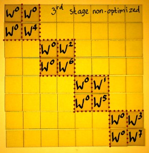 |
On the left I have written all rotations as positive powers of
W. The series is: W0 W4 W2 W6 W1 W5 W3 W7 This is a pattern we have seen before. It is bit-reversed. Of course, this will have a different meaning in every stage of the FFT. The 8th roots of unity have three bits, the 4th roots have two bits, and the square roots have one bit. |
So in this scheme we have to apply the twiddle factors in bit-reversed order, and the output is also in bit-reversed order. Then the question arises if the twiddle factors can be used in their natural order, to have the output in natural order as well. I have tried that, just for curiosity. If it would work, everyone would use that of course. But it does not work. Decimation is the essence of FFT. Recall that downsampling is also a form of rotation. It doubles a frequency everytime. As such it is part of the strategy for getting all rotation factors at their proper position. Without it, output bin number 1 for example would have these nonsense values:
x[0]+x[4]+x[2]+x[6] + (x[1]+x[5]+x[3]+x[7])*W1
Downsampling W1 gives W2, and downsampling one more time gives W4. Then it makes sense, being the correlation output of harmonic number 4.
x[0]+x[4]+x[2]+x[6] + (x[1]+x[5]+x[3]+x[7])*W4
Decimation brings us to subsequent schemes, in which the input signal is reorganised with indexes bit-reversed, before all other operations. The output will appear with the frequencies in natural order.
 |
 |
 |
 |
This scheme has 'first-twiddle-then-add&subtract'. As an example, I sketch the third FFT stage here below, because in the other ones there is less to see. The twiddle factors appear in their natural order.
 |
 |
|
There is one more regular radix 2 form with the input decimated:
 |
 |
 |
|
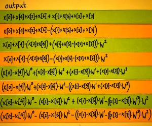
In this scheme the additions/subtractions are done before the twiddling. Now I choose the first stage for illustration. The twiddle factors do not appear in their natural order. One would quickly guess what happened to the order...
 |
|
|
These were the four basic radix 2 FFT forms, illustrated for N=8. Modifications of them are conceivable, for instance a phase reordering inbetween each stage, to have input and output in natural order directly.
For convenience, the tables of the four schemes are showed once more, next to each other.
1. decimated spectrum:
|
|
|
|
2. decimated spectrum / decimated W series:
|
|
|
|
3. decimated input:
|
|
|
|
4. decimated input / decimated W series:
|
|
|
|
FFT in C
Now that I learned how a Fourier matrix can be decomposed into radix 2 FFT factors, the next challenge is to implement this in a computer language. After all, outside a computer even the optimallest Fast Fourier Transform is of little practical use. Although the first invention of the technique dates from the early nineteenth century...
Below is the sketch of a radix 2 FFT for N=8, as it was figured out on preceding pages, and from which I will depart:
 |
 |
 |
 |
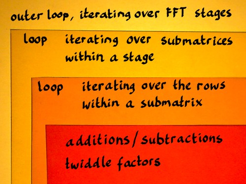
A routine for this FFT could or should be organised as a series of nested loops. I have seen this principle outlined in texts on FFT, notably in The Fast Fourier Transform by E. Oran Brigham, Numerical Recipes in C by William H. Press e.a., and Kevin 'fftguru' McGee's online FFT tutorial. The point is that I had a hard time to understand the mechanics of it. So I went step by step, studying texts and code, and working out my coloured square paper models in parallel. FFT was like a jig saw puzzle for me, and this page reflects how I was putting the pieces together.
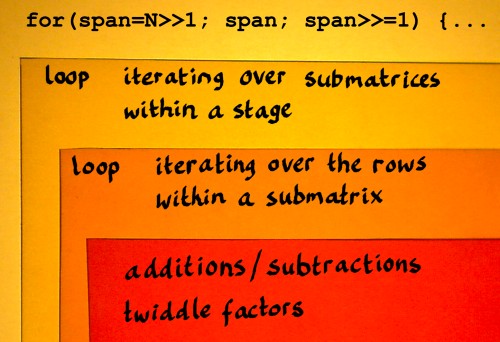
In the matrix representation, the structure of an FFT shows several layers:
- the sparse factor matrices representing the FFT stages
- submatrices appearing in each factor matrix
- row entries appearing pairwise in each submatrix
An FFT implementation can be organised accordingly, and for the moment I will just sketch that roughly:
 |
When we look at the FFT factor matrices, there is a kind of virtual vector size that is smaller and smaller in each consecutive stage. In the first stage, this size is N/2 and in the last stage it is reduced to just 1.
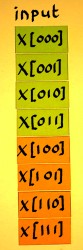
I feel that we should inspect the indexes in their binary form for a moment. Binary integer numbers are what computers use internally for indexing, which in turn is an incentive to do radix 2 FFT. If there is a pattern to perceive, it is best perceived in the binary numbers. Here is the addition/subtraction matrix of the first stage, with all indexes written in binary:
 |
 |
 |
N/2 can also be defined N>>1, which means N shifted right by one bit: 1000 becomes 0100. It is a pure power of two everytime. Instead of using 4 as a constant, or writing N/2 a couple of times, it would be efficient to store the value in some variable, and update it in every stage. I will label this variable 'span', as that seems an appropriate title for this essential parameter.
 |
 |
 |
We can declare span as a variable of datatype unsigned int, and initialize it at the start of the outer loop:
span = N>>1;
Span can be decremented in appropriate steps for the iterations over the FFT stages:
span >>= 1;
From 0100 it will shift to 0010 in the second stage and to 0001 in the third stage. After that it will shift right from 0001 to 0000, which is also boolean 'false'. That is where the outer loop should end indeed. Therefore the variable span can also regulate the conditions for the outer loop.
Let me insert this into the rough FFT sketch, in C manner:
 |
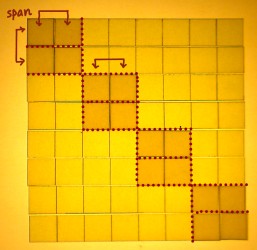
Index numbers can now be referenced as x[n] and x[n+span]. That is how we can identify sample pairs for addition/subtraction. This identification method will only run smooth when the work will be done on one submatrix at a time, within each stage. Otherwise x[n] will overlap with x[n+span]. We could write a for-loop that iterates over the submatrices in a stage.
 |
Every stage has it's own amount of submatrices. The first stage has just one NxN matrix. The second stage shows two submatrices. The third stage has four submatrices. The amount of submatrices in each stage is inversely proportional to span. More precisely, it is N/(span*2) or (N>>1)/span. Our for-loop can be something like:
|
start with submatrix=0; continue as long as the value of submatrix is smaller than (N>>1)/span; increment submatrix with 1 after each iteration; |
Adding these considerations to the FFT plan:
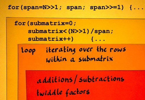 |
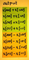
Within each submatrix we have to perform addition/subtraction and compute output pairs of the following kind:
|
x[n]+x[n+span]; x[n]-x[n+span]; // the latter output to be twiddled |
I have seen such pairs being called 'dual node pairs', in Oran Brigham's book 'the Fast Fourier Transform'. There, the term applies to points where things come together in a butterfly figure. There is no butterflies here, but I like the term. Let me identify such a dual node pair like it shall be computed in the first FFT stage:
 |
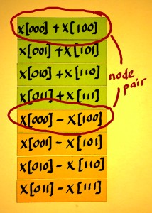
|
We bring x[000] and x[100] together, and perform addition of these on one hand, and subtraction on the other hand. After that, the results go their own way again. |
How many dual node pairs do we have in a submatrix? There is already a variable that has the correct value: span. We can iterate over the dual node pairs using a straightforward loop that I will add to my preliminary scheme:
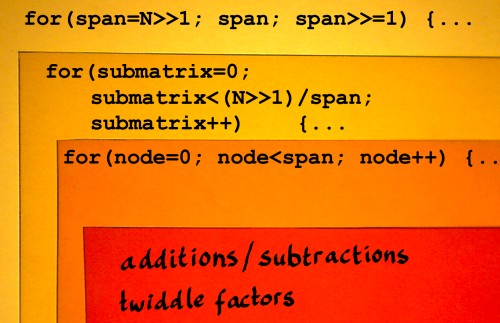 |
After finishing the iterations over the nodes, n has to jump over the x[n+span] values. But it must not get bigger than N. It can be done like: n=(n+span)&(N-1). The &(N-1) is a bitwise-and mask, for example: binary 11111 is such a mask in the N=32 case.
Until here I have three for-loops written down, but all the work of calculating the content still has to be done. What a crazy routine it is... Let me then see how to handle the additions/subtractions of the dual node pairs:
|
x[n]=x[n]+x[n+span]; x[n+span]=x[n]-x[n+span]; // these shall be twiddled |
Aha. Here is a small problem: in this way the original value of x[n] can not be used for the computation of x[n+span], as it is already overwritten in the first line. Unfortunately, a temporary variable is needed to store the new value for x[n] for a short while:
|
temp=x[n]+x[n+span]; x[n+span]=x[n]-x[n+span]; x[n]=temp; |
This is all still quite theoretical, because x[n] is a complex variable in real life. Let us split x[n] in real[n] and im[n] for the moment, and check how the code could expand:
|
temp=real[n]+real[n+span]; real[n+span]=real[n]-real[n+span]; real[n]=temp; temp=im[n]+im[n+span]; im[n+span]=im[n]-im[n+span]; im[n]=temp; |
Now it turns out that for each n, the value [n+span] is already computed six times. Shall I not store this value before the additions and subtractions, in a variable called nspan? (Yep).
What comes next? We need to multiply the x[nspan] output values with twiddle factors. This is best done while these output values are still at hand, in the CPU registers (hopefully) or else somewhere nearby in cache. The twiddling is therefore inside the loop over the nodes, the innerest loop. Directly after the subtraction x[nspan]=x[n]-x[nspan], x[nspan] can be updated with the twiddle factor. Again, this is somewhat more complicated in real life, as it concerns a complex multiplication. And furthermore, we do not have these twiddle factors computed yet. So here I really have to start a new topic.
Twiddling
The twiddle factors shall be square roots of unity and square roots thereof, etcetera, related to each stage. Our N=8 FFT starts with the eight-roots of unity. The angle in radians for the primitive eight-root of unity, the first interval, could be computed with -2pi/8. But we have this handy variable span, initialized at N/2 and updated for each FFT stage. Therefore, angle of the primitive root for each stage can be computed as: -pi/span. So span functions as a complex root extractor, cool... This primitive root angle has to be updated for each new iteration within the outer loop:
|
primitive_root = MINPI/span; // define MINPI
in the header |
If this root angle is multiplied with the node variable in the innerest loop, we have the correct angle for every twiddle factor:
|
angle = primitive_root * node; |
From this angle, sine and cosine must be computed. That could simply be done like:
|
realtwiddle = cos(angle); imtwiddle = sin(angle); |
I will postpone my comments on this till later, let me first try to finish the routine. real[nspan] and im[nspan] need complex multiplication with realtwiddle and imtwiddle. Again, a temporary variable is inevitable:
|
temp = realtwiddle * real[nspan] - imtwiddle * im[nspan]; im[nspan] = realtwiddle * im[nspan] + imtwiddle * real[nspan]; real[nspan] = temp; |
For the next node, n must be incremented. We're done! Let me now put these codebits together.
|
void FFT(unsigned int logN, double *real, double *im) // logN is base 2 log(N) { unsigned int n=0, nspan, span, submatrix, node; unsigned int N = 1<<logN; double temp, primitive_root, angle, realtwiddle, imtwiddle; for(span=N>>1; span; span>>=1) // loop over the FFT stages { primitive_root = MINPI/span; // define MINPI in the header for(submatrix=0; submatrix<(N>>1)/span; submatrix++) { for(node=0; node<span; node++) { nspan = n+span; temp = real[n] + real[nspan]; // additions & subtractions real[nspan] = real[n]-real[nspan]; real[n] = temp; temp = im[n] + im[nspan]; im[nspan] = im[n] - im[nspan]; im[n] = temp; angle = primitive_root * node; // rotations realtwiddle = cos(angle); imtwiddle = sin(angle); temp = realtwiddle * real[nspan] - imtwiddle * im[nspan]; im[nspan] = realtwiddle * im[nspan] + imtwiddle * real[nspan]; real[nspan] = temp; n++; // not forget to increment n } // end of loop over nodes n = (n+span) & (N-1); // jump over the odd blocks } // end of loop over submatrices } // end of loop over FFT stages } // end of FFT function |
With some twenty lines of C code we can have an FFT function. The output of this FFT appears in bit-reversed order, so for analysis purposes it does not make much sense yet. I will figure out bitreversal on a separate page. Furthermore, the output is not normalised in any way.
Of course, this simple FFT code is still highly inefficient. The real killer is: the calling of standard trigonometrics, cos() and sin(). Why is that so? For one thing, the hardware FPU trig instructions generate 80 bits precision output by default. They really take a lot of clock cycles. If we are to optimize the code, here is the obvious point to start. The next page shows some modifications.
No hay comentarios:
Publicar un comentario