Numerical Analysis in Python, Tutorial and Online Course

http://www.python-course.eu/numerical_programming.php

Tutorial and Online Course

Data Science and Data Analysis

Comment on our own account: Since October 2015 we are working on this tutorial on numerical programming in Python. Since then it has been the focus of our work. On the 10th of February 2016, we started translating the documentation into German..

This is a tutorial, which can be used as an online course on Data Science and Data Analysis. Data Analysis is widely understood as the science of managing and anlysing large datasets, or Big Data. It also means providing the tools to inspect, transform and model data. The goal mainly consists in gaining information.

An Alternative to Matlab

Many scientists and engineers in the scientific and engineering world use R and MATLAB to solve their data analysis and data science problems. It's a question troubling lots of people, which language they should choose: The functionality of R was developed with statisticians in mind, whereas Python is a general-purpose language. Nevertheless, Python is also - in combination with its specialized modules, like Numpy, Scipy, Matplotlib, Pandas and so, - an ideal programming language for solving numerical problems. Furthermore, the community of Python is a lot larger and faster growing than the one from R. The principal disadvantage of MATLAB against Python are the costs. Python is completely free, whereas MATLAB can be very expensive. Python is a very attractive alternative of MATLAB: Python is not only free of costs, but its code is open source. Python is continually becoming more powerful by a rapidly growing number of specialized modules. Python in combination with Numpy, Scipy and Matplotlib can be used as a replacement for MATLAB. The combination of NumPy, SciPy and Matplotlib is a free (meaning both "free" as in "free beer" and "free" as in "freedom") alternative to MATLAB. Even though MATLAB has a huge number of additional toolboxes available, NumPy has the advantage that Python is a more modern and complete programming language and - as we have said already before - is open source. SciPy adds even more MATLAB-like functionalities to Python. Python is rounded out in the direction of MATLAB with the module Matplotlib, which provides MATLAB-like plotting functionality.

Data Anaysis

Numpy Tutorial

Introduction

NumPy is an acronym for "Numeric Python" or "Numerical Python". It is an open source extension module for Python, which provides fast precompiled functions for mathematical and numerical routines. Furthermore, NumPy enriches the programming language Python with powerful data structures for efficient computation of multi-dimensional arrays and matrices. The implementation is even aiming at huge matrices and arrays. Besides that the module supplies a large library of high-level mathematical functions to operate on these matrices and arrays.
SciPy (Scientific Python) is often mentioned in the same breath with NumPy. SciPy extends the capabilities of NumPy with further useful functions for minimization, regression, Fourier-transformation and many others.
Both NumPy and SciPy are usually not installed by default. NumPy has to be installed before installing SciPy. Numpy can be downloaded from the website:
http://www.numpy.org
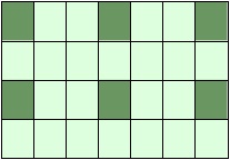
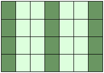
(Comment: The diagram of the image on the right side is the graphical visualisation of a matrix with 14 rows and 20 columns. It's a so-called Hinton diagram. The size of a square within this diagram corresponds to the size of the value of the depicted matrix. The colour determines, if the value is positive or negative. In our example: the colour red denotes negative values and the colour green denotes positive values.)
NumPy is based on two earlier Python modules dealing with arrays. One of these is Numeric. Numeric is like NumPy a Python module for high-performance, numeric computing, but it is obsolete nowadays. Another predecessor of NumPy is Numarray, which is a complete rewrite of Numeric but is deprecated as well. NumPy is a merger of those two, i.e. it is build on the code of Numeric and the features of Numarray.

The Python Alternative to Matlab

Python in combination with Numpy, Scipy and Matplotlib can be used as a replacement for MATLAB. The combination of NumPy, SciPy and Matplotlib is a free (meaning both "free" as in "free beer" and "free" as in "freedom") alternative to MATLAB. Even though MATLAB has a huge number of additional toolboxes available, NumPy has the advantage that Python is a more modern and complete programming language and - as we have said already before - is open source. SciPy adds even more MATLAB-like functionalities to Python. Python is rounded out in the direction of MATLAB with the module Matplotlib, which provides MATLAB-like plotting functionality.

Comparison between Core Python and Numpy

When we say "Core Python", we mean Python without any special modules, i.e. especially without NumPy.
The advantages of Core Python:

• high-level number objects: integers, floating point
• containers: lists with cheap insertion and append methods, dictionaries with fast lookup

Advantages of using Numpy with Python:

• array oriented computing
• efficiently implemented multi-dimensional arrays
• designed for scientific computation

A Simple Numpy Example

Before we can use NumPy we will have to import it. It has to be imported like any other module:

import numpy

But you will hardly ever see this. Numpy is usually renamed to np:

import numpy as np

We have a list with values, e.g. temperatures in Celsius:

cvalues = [25.3, 24.8, 26.9, 23.9]

We will turn this into a one-dimensional numpy array:

C = np.array(cvalues)
print(C)

[ 25.3  24.8  26.9  23.9]

Let's assume, we want to turn the values into degrees Fahrenheit. This is very easy to accomplish with a numpy array. The solution to our problem can be achieved by simple scalar multiplication:

print(C * 9 / 5 + 32)

[ 77.54  76.64  80.42  75.02]

Compared to this, the solution for our Python list is extremely awkward:

fvalues = [ x*9/5 + 32 for x in cvalues] 
print(fvalues)

[77.54, 76.64, 80.42, 75.02]

Creation of Evenly Spaced Values

There are functions provided by Numpy to create evenly spaced values within a given interval. One uses a given distance 'arange' and the other one 'linspace' needs the number of elements and creates the distance automatically.

arange

The syntax of arange:
arange([start,] stop[, step,], dtype=None)
arange returns evenly spaced values within a given interval. The values are generated within the half-open interval '[start, stop)' If the function is used with integers, it is nearly equivalent to the Python built-in function range, but arange returns an ndarray rather than a list iterator as range does. If the 'start' parameter is not given, it will be set to 0. The end of the interval is determined by the parameter 'stop'. Usually, the interval will not include this value, except in some cases where 'step' is not an integer and floating point round-off affects the length of output ndarray. The spacing between two adjacent values of the output array is set with the optional parameter 'step'. The default value for 'step' is 1. If the parameter 'step' is given, the 'start' parameter cannot be optional, i.e. it has to be given as well. The type of the output array can be specified with the parameter 'dtype'. If it is not given, the type will be automatically inferred from the other input arguments.

import numpy as np
a = np.arange(1, 10)
print(a)
# compare to range:
x = range(1,10)
print(x)    # x is an iterator
print(list(x))
# some more arange examples:
x = np.arange(10.4)
print(x)
x = np.arange(0.5, 10.4, 0.8)
print(x)
x = np.arange(0.5, 10.4, 0.8, int)
print(x)

[1 2 3 4 5 6 7 8 9]
range(1, 10)
[1, 2, 3, 4, 5, 6, 7, 8, 9]
[  0.   1.   2.   3.   4.   5.   6.   7.   8.   9.  10.]
[  0.5   1.3   2.1   2.9   3.7   4.5   5.3   6.1   6.9   7.7   8.5   9.3
  10.1]
[ 0  1  2  3  4  5  6  7  8  9 10 11 12]

linspace

The syntax of linspace:
linspace(start, stop, num=50, endpoint=True, retstep=False)
linspace returns an ndarray, consisting of 'num' equally spaced samples in the closed interval [start, stop] or the half-open interval [start, stop). If a closed or a half-open interval will be returned, depends on whether 'endpoint' is True or False. The parameter 'start' defines the start value of the sequence which will be created. 'stop' will the end value of the sequence, unless 'endpoint' is set to False. In the latter case, the resulting sequence will consist of all but the last of 'num + 1' evenly spaced samples. This means that 'stop' is excluded. Note that the step size changes when 'endpoint' is False. The number of samples to be generated can be set with 'num', which defaults to 50. If the optional parameter 'endpoint' is set to True (the default), 'stop' will be the last sample of the sequence. Otherwise, it is not included.

import numpy as np
# 50 values between 1 and 10:
print(np.linspace(1, 10))
# 7 values between 1 and 10:
print(np.linspace(1, 10, 7))
# excluding the endpoint:
print(np.linspace(1, 10, 7, endpoint=False))

[  1.           1.18367347   1.36734694   1.55102041   1.73469388
   1.91836735   2.10204082   2.28571429   2.46938776   2.65306122
   2.83673469   3.02040816   3.20408163   3.3877551    3.57142857
   3.75510204   3.93877551   4.12244898   4.30612245   4.48979592
   4.67346939   4.85714286   5.04081633   5.2244898    5.40816327
   5.59183673   5.7755102    5.95918367   6.14285714   6.32653061
   6.51020408   6.69387755   6.87755102   7.06122449   7.24489796
   7.42857143   7.6122449    7.79591837   7.97959184   8.16326531
   8.34693878   8.53061224   8.71428571   8.89795918   9.08163265
   9.26530612   9.44897959   9.63265306   9.81632653  10.        ]
[  1.    2.5   4.    5.5   7.    8.5  10. ]
[ 1.          2.28571429  3.57142857  4.85714286  6.14285714  7.42857143
  8.71428571]

We haven't discussed one interesting parameter so far. If the optional parameter 'retstep' is set, the function will also return the value of the spacing between adjacent values. So, the function will return a tuple ('samples', 'step'):

import numpy as np
samples, spacing = np.linspace(1, 10, retstep=True)
print(spacing)
samples, spacing = np.linspace(1, 10, 20, endpoint=True, retstep=True)
print(spacing)
samples, spacing = np.linspace(1, 10, 20, endpoint=False, retstep=True)
print(spacing)

0.1836734693877551
0.47368421052631576
0.45

Time Comparison between Python Lists and Numpy Arrays

One of the main advantages of NumPy is its advantage in time compared to standard Python. Let's look at the following functions:

import time
size_of_vec = 1000
def pure_python_version():
    t1 = time.time()
    X = range(size_of_vec)
    Y = range(size_of_vec)
    Z = []
    for i in range(len(X)):
        Z.append(X[i] + Y[i])
    return time.time() - t1
def numpy_version():
    t1 = time.time()
    X = np.arange(size_of_vec)
    Y = np.arange(size_of_vec)
    Z = X + Y
    return time.time() - t1

Let's call these functions and see the time consumption:

t1 = pure_python_version()
t2 = numpy_version()
print(t1, t2)
print("Numpy is in this example " + str(t1/t2) + " faster!")

0.0002090930938720703 2.0503997802734375e-05
Numpy is in this example 10.19767441860465 faster!

It's an easier and above all better way to measure the times by using the timeit module. We will use the Timer class in the following script.
The constructor of a Timer object takes a statement to be timed, an additional statement used for setup, and a timer function. Both statements default to 'pass'.
The statements may contain newlines, as long as they don't contain multi-line string literals.

import numpy as np
from timeit import Timer
size_of_vec = 1000
def pure_python_version():
    X = range(size_of_vec)
    Y = range(size_of_vec)
    Z = []
    for i in range(len(X)):
        Z.append(X[i] + Y[i])
def numpy_version():
    X = np.arange(size_of_vec)
    Y = np.arange(size_of_vec)
    Z = X + Y
#timer_obj = Timer("x = x + 1", "x = 0")
timer_obj1 = Timer("pure_python_version()", "from __main__ import pure_python_version")
timer_obj2 = Timer("numpy_version()", "from __main__ import numpy_version")
print(timer_obj1.timeit(10))
print(timer_obj2.timeit(10))

0.0022348780039465055
6.224898970685899e-05

Creating Arrays

Zero-dimensional Arrays in Numpy

It's possible to create multidimensional arrays in numpy. Scalars are zero dimensional. In the following example, we will create the scalar 42. Applying the ndim method to our scalar, we get the dimension of the array. We can also see that the type is a "numpy.ndarray" type.

import numpy as np
x = np.array(42)
print("x: ", x)
print("The type of x: ", type(x))
print("The dimension of x:", np.ndim(x))

x:  42
The type of x:  <class 'numpy.ndarray'>
The dimension of x: 0

One-dimensional Arrays

We have already encountered a 1-dimenional array - better known to some as vectors - in our initial example. What we have not mentioned so far, but what you may have assumed, is the fact that numpy arrays are containers of items of the same type, e.g. only integers. The homogenous type of the array can be determined with the attribute "dtype", as we can learn from the following example:

F = np.array([1, 1, 2, 3, 5, 8, 13, 21])
V = np.array([3.4, 6.9, 99.8, 12.8])
print("F: ", F)
print("V: ", V)
print("Type of F: ", F.dtype)
print("Type of V: ", V.dtype)
print("Dimension of F: ", np.ndim(F))
print("Dimension of V: ", np.ndim(V))

F:  [ 1  1  2  3  5  8 13 21]
V:  [  3.4   6.9  99.8  12.8]
Type of F:  int64
Type of V:  float64
Dimension of F:  1
Dimension of V:  1

Two- and Multidimensional Arrays

Of course, arrays of NumPy are not limited to one dimension. They are of arbitrary dimension. We create them by passing nested lists (or tuples) to the array method of numpy.

A = np.array([ [3.4, 8.7, 9.9], 
               [1.1, -7.8, -0.7],
               [4.1, 12.3, 4.8]])
print(A)
print(A.ndim)

[[  3.4   8.7   9.9]
 [  1.1  -7.8  -0.7]
 [  4.1  12.3   4.8]]
2

B = np.array([ [[111, 112], [121, 122]],
               [[211, 212], [221, 222]],
               [[311, 312], [321, 322]] ])
print(B)
print(B.ndim)

[[[111 112]
  [121 122]]
 [[211 212]
  [221 222]]
 [[311 312]
  [321 322]]]
3

Shape of an Array

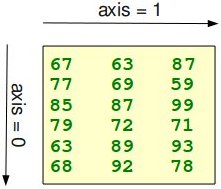
The function "shape" returns the shape of an array. The shape is a tuple of integers. These numbers denote the lengths of the corresponding array dimension. In other words: The "shape" of an array is a tuple with the number of elements per axis (dimension). In our example, the shape is equal to (6, 3), i.e. we have 6 lines and 3 columns.

x = np.array([ [67, 63, 87],
               [77, 69, 59],
               [85, 87, 99],
               [79, 72, 71],
               [63, 89, 93],
               [68, 92, 78]])
print(np.shape(x))

(6, 3)

There is also an equivalent array property:

print(x.shape)

(6, 3)

The shape of an array tells us also something about the order in which the indices are processed, i.e. first rows, then columns and after that the further dimensions.
"shape" can also be used to change the shape of an array.

x.shape = (3, 6)
print(x)

[[67 63 87 77 69 59]
 [85 87 99 79 72 71]
 [63 89 93 68 92 78]]

x.shape = (2, 9)
print(x)

[[67 63 87 77 69 59 85 87 99]
 [79 72 71 63 89 93 68 92 78]]

You might have guessed by now that the new shape must correspond to the number of elements of the array, i.e. the total size of the new array must be the same as the old one. We will raise an exception, if this is not the case:

x.shape = (4, 4)

We received the following result:

---------------------------------------------------------------------------
ValueError                                Traceback (most recent call last)
<ipython-input-81-5c4497921b8c> in <module>()
----> 1 x.shape = (4, 4)
ValueError: total size of new array must be unchanged

Let's look at some further examples.
The shape of a scalar is an empty tuple:

x = np.array(11)
print(np.shape(x))

()

B = np.array([ [[111, 112], [121, 122]],
               [[211, 212], [221, 222]],
               [[311, 312], [321, 322]] ])
print(B.shape)

(3, 2, 2)

Indexing and Slicing

Assigning to and accessing the elements of an array is similar to other sequential data types of Python, i.e. lists and tuples. We have also many options to indexing, which makes indexing in Numpy very powerful and similar to core Python.
Single indexing is the way, you will most probably expect it:

F = np.array([1, 1, 2, 3, 5, 8, 13, 21])
# print the first element of F, i.e. the element with the index 0
print(F[0])
# print the last element of F
print(F[-1])
B = np.array([ [[111, 112], [121, 122]],
               [[211, 212], [221, 222]],
               [[311, 312], [321, 322]] ])
print(B[0][1][0])

1
21
121

Indexing multidimensional arrays:

A = np.array([ [3.4, 8.7, 9.9], 
               [1.1, -7.8, -0.7],
               [4.1, 12.3, 4.8]])
print(A[1][0])

1.1

We accessed the element in the second row, i.e. the row with the index 1, and the first column (index 0). We accessed it the same way, we would have done with an element of a nested Python list. There is another way to access elements of multidimensional arrays in numpy.
There is also an alternative: We use only one pair of square brackets and all the indices are separated by commas:

print(A[1, 0])

1.1

You have to be aware of the fact, that the second way is more efficient. In the first case, we create an intermediate array A[1] from which we access the element with the index 0. So it behaves similar to this:

tmp = A[1]
print(tmp)
print(tmp[0])

[ 1.1 -7.8 -0.7]
1.1

We assume that you are familar with the slicing of lists and tuples. The syntax is the same in numpy for one-dimensional arrays, but it can be applied to multiple dimensions as well.
The general syntax for a one-dimensional array A looks like this:
A[start:stop:step]
We illustrate the operating principle of "slicing" with some examples. We start with the easiest case, i.e. the slicing of a one-dimensional array:

S = np.array([0, 1, 2, 3, 4, 5, 6, 7, 8, 9])
print(S[2:5])
print(S[:4])
print(S[6:])
print(S[:])

[2 3 4]
[0 1 2 3]
[6 7 8 9]
[0 1 2 3 4 5 6 7 8 9]

We will illustrate the multidimensional slicing in the following examples. The ranges for each dimension are separated by commas:

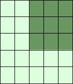
A = np.array([
[11,12,13,14,15],
[21,22,23,24,25],
[31,32,33,34,35],
[41,42,43,44,45],
[51,52,53,54,55]])
print(A[:3,2:])

[[13 14 15]
 [23 24 25]
 [33 34 35]]

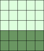
print(A[3:,:])

[[41 42 43 44 45]
 [51 52 53 54 55]]

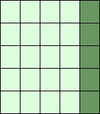
print(A[:,4:])

[[15]
 [25]
 [35]
 [45]
 [55]]

The following two examples use the third parameter "step". The reshape function is used to construct the two-dimensional array. We will explain reshape in the following subchapter:

X = np.arange(28).reshape(4,7)
print(X)

[[ 0  1  2  3  4  5  6]
 [ 7  8  9 10 11 12 13]
 [14 15 16 17 18 19 20]
 [21 22 23 24 25 26 27]]

print(X[::2, ::3])

[[ 0  3  6]
 [14 17 20]]

print(X[::, ::3])

[[ 0  3  6]
 [ 7 10 13]
 [14 17 20]
 [21 24 27]]

Attention: Whereas slicings on lists and tuples create new objects, a slicing operation on an array creates a view on the original array. So we get an another possibility to access the array, or better a part of the array. From this follows that if we modify a view, the original array will be modified as well.

A = np.array([0, 1, 2, 3, 4, 5, 6, 7, 8, 9])
S = A[2:6]
S[0] = 22
S[1] = 23
print(A)

[ 0  1 22 23  4  5  6  7  8  9]

Doing the similar thing with lists, we can see that we get a copy:

lst = [0, 1, 2, 3, 4, 5, 6, 7, 8, 9]
lst2 = lst[2:6]
lst2[0] = 22
lst2[1] = 23
print(lst)

[0, 1, 2, 3, 4, 5, 6, 7, 8, 9]

If you want to check, if two array names share the same memory block, you can use the function np.may_share_memory.
np.may_share_memory(A, B)
To determine if two arrays A and B can share memory the memory-bounds of A and B are computed. The function returns True, if they overlap and False otherwise. The function may give false positives, i.e. if it returns True it just means that the arrays may be the same.

np.may_share_memory(A, S)

This gets us the following:

True

The following code shows a case, in which the use of may_share_memory is quite useful:

A = np.arange(12)
B = A.reshape(3, 4)
A[0] = 42
print(B)

[[42  1  2  3]
 [ 4  5  6  7]
 [ 8  9 10 11]]

We can see that A and B share the memory in some way. The array attribute "data" is an object pointer to the start of an array's data. Looking at the data attribute returns something surprising:

print(A.data)
print(B.data)
print(A.data == B.data)

<memory at 0x7fe3b458dd90>
<memory at 0x7fe3b45a9e48>
False

Let's check now on equality of the arrays:

print(A == B)

False

Which makes sense, because they are different arrays concerning their structure:

print(A)
print(B)

[42  1  2  3  4  5  6  7  8  9 10 11]
[[42  1  2  3]
 [ 4  5  6  7]
 [ 8  9 10 11]]

But we saw that if we change an element of one array the other one is changed as well. This fact is reflected by may_share_memory:

np.may_share_memory(A, B)

The above code returned the following output:

True

The result above is "false positive" example for may_share_memory in the sense that somebody may think that the arrays are the same, which is not the case.

Arrays of Ones and of Zeros

There are two ways of initializing Arrays with Zeros or Ones. The method ones(t) takes a tuple t with the shape of the array and fills the array accordingly with ones. By default it will be filled with Ones of type float. If you need integer Ones, you have to set the optional parameter dtype to int:

import numpy as np
E = np.ones((2,3))
print(E)
F = np.ones((3,4),dtype=int)
print(F)

[[ 1.  1.  1.]
 [ 1.  1.  1.]]
[[1 1 1 1]
 [1 1 1 1]
 [1 1 1 1]]

What we have said about the method ones() is valid for the method zeros() analogously, as we can see in the following example:

Z = np.zeros((2,4))
print(Z)

[[ 0.  0.  0.  0.]
 [ 0.  0.  0.  0.]]

There is another interesting way to create an array with Ones or with Zeros, if it has to have the same shape as another existing array 'a'. Numpy supplies for this purpose the methods ones_like(a) and zeros_like(a).

x = np.array([2,5,18,14,4])
E = np.ones_like(x)
print(E)
Z = np.zeros_like(x)
print(Z)

[1 1 1 1 1]
[0 0 0 0 0]

Copying Arrays

numpy.copy()

copy(obj, order='K')
Return an array copy of the given object 'obj'.

Parameter	Meaning
obj	array_like input data.
order	The possible values are {'C', 'F', 'A', 'K'}. This parameter controls the memory layout of the copy. 'C' means C-order, 'F' means Fortran-order, 'A' means 'F' if the object 'obj' is Fortran contiguous, 'C' otherwise. 'K' means match the layout of 'obj' as closely as possible.

import numpy as np
x = np.array([[42,22,12],[44,53,66]], order='F')
y = x.copy()
x[0,0] = 1001
print(x)
print(y)

[[1001   22   12]
 [  44   53   66]]
[[42 22 12]
 [44 53 66]]

print(x.flags['C_CONTIGUOUS'])
print(y.flags['C_CONTIGUOUS'])

False
True

ndarray.copy()

There is also a ndarray method 'copy', which can be directly applied to an array. It is similiar to the above function, but the default values for the order arguments are different.
a.copy(order='C')
Returns a copy of the array 'a'.

Parameter	Meaning
order	The same as with numpy.copy, but 'C' is the default value for order.

import numpy as np
x = np.array([[42,22,12],[44,53,66]], order='F')
y = x.copy()
x[0,0] = 1001
print(x)
print(y)
print(x.flags['C_CONTIGUOUS'])
print(y.flags['C_CONTIGUOUS'])

[[1001   22   12]
 [  44   53   66]]
[[42 22 12]
 [44 53 66]]
False
True

Identity Array

An identity array is a square array with ones on its main diagonal. There are two ways to create identity array.

• identy
• eye

The identity Function

We can create identity arrays with the function identity:
identity(n, dtype=None)
The parameters:

Parameter	Meaning
n	An integer number defining the number of rows and columns of the output, i.e. 'n' x 'n'
dtype	An optional argument, defining the data-type of the output. The default is 'float'

The output of identity is an 'n' x 'n' array with its main diagonal set to one, and all other elements are 0.

import numpy as np
np.identity(4)

The code above returned the following:

array([[ 1.,  0.,  0.,  0.],
       [ 0.,  1.,  0.,  0.],
       [ 0.,  0.,  1.,  0.],
       [ 0.,  0.,  0.,  1.]])

np.identity(4, dtype=int) # equivalent to np.identity(3, int)

This gets us the following:

array([[1, 0, 0, 0],
       [0, 1, 0, 0],
       [0, 0, 1, 0],
       [0, 0, 0, 1]])

The eye Function

Another way to create identity arrays provides the function eye. It returns a 2-D array with ones on the diagonal and zeros elsewhere.
eye(N, M=None, k=0, dtype=float)

Parameter	Meaning
N	An integer number defining the rows of the output array.
M	An optional integer for setting the number of columns in the output. If it is None, it defaults to 'N'.
k	Defining the position of the diagonal. The default is 0. 0 refers to the main diagonal. A positive value refers to an upper diagonal, and a negative value to a lower diagonal.
dtype	Optional data-type of the returned array.

eye returns an ndarray of shape (N,M). All elements of this array are equal to zero, except for the 'k'-th diagonal, whose values are equal to one.

import numpy as np
np.eye(5, 8, k=1, dtype=int)

The above Python code returned the following:

array([[0, 1, 0, 0, 0, 0, 0, 0],
       [0, 0, 1, 0, 0, 0, 0, 0],
       [0, 0, 0, 1, 0, 0, 0, 0],
       [0, 0, 0, 0, 1, 0, 0, 0],
       [0, 0, 0, 0, 0, 1, 0, 0]])

The principle of operation of the parameter 'd' of the eye function is illustrated in the following diagram:

Exercises:

1) Create an arbitrary one dimensional array called "v".
2) Create a new array which consists of the odd indices of previously created array "v".
3) Create a new array in backwards ordering from v.
4) What will be the output of the following code:

   a = np.array([1, 2, 3, 4, 5])
   b = a[1:4]
   b[0] = 200
   print(a[1])
   

5) Create a two dimensional array called "m".
6) Create a new array from m, in which the elements of each row are in reverse order.
7) Another one, where the rows are in reverse order.
8) Create an array from m, where columns and rows are in reverse order.
9) Cut of the first and last row and the first and last column.

Solutions to the Exercises:

1)

   import numpy as np
   a = np.array([3,8,12,18,7,11,30])
   

2)

odd_elements = a[1::2]

3) reverse_order = a[::-1]
4) The output will be 200, because slices are views in numpy and not copies.
5) m = np.array([ [11, 12, 13, 14], [21, 22, 23, 24], [31, 32, 33, 34]])
6) m[::,::-1]
7) m[::-1]
8) m[::-1,::-1]
9) m[1:-1,1:-1]