https://ataspinar.com/2018/12/21/a-guide-for-using-the-wavelet-transform-in-machine-learning/
A guide for using the Wavelet Transform in Machine Learning
1. Introduction
In a previous blog-post we have seen how we can use Signal Processing techniques for the classification of time-series and signals.
A very short summary of that post is: We can use the Fourier Transform to transform a signal from its time-domain to its frequency domain. The peaks in the frequency spectrum indicate the most occurring frequencies in the signal. The larger and sharper a peak is, the more prevalent a frequency is in a signal. The location (frequency-value) and height (amplitude) of the peaks in the frequency spectrum then can be used as input for Classifiers like Random Forest or Gradient Boosting.
This simple approach works surprisingly well for many classification problems. In that blog post we were able to classify the Human Activity Recognition dataset with a ~91 % accuracy.
The general rule is that this approach of using the Fourier Transform will work very well when the frequency spectrum is stationary. That is, the frequencies present in the signal are not time-dependent; if a signal contains a frequency of x  this frequency should be present equally anywhere in the signal.
The more non-stationary/dynamic a signal is, the worse the results will be. That’s too bad, since most of the signals we see in real life are non-stationary in nature. Whether we are talking about ECG signals, the stock market, equipment or sensor data, etc, etc, in real life problems start to get interesting when we are dealing with dynamic systems. A much better approach for analyzing dynamic signals is to use the Wavelet Transform instead of the Fourier Transform.
Even though the Wavelet Transform is a very powerful tool for the analysis and classification of time-series and signals, it is unfortunately not known or popular within the field of Data Science. This is partly because you should have some prior knowledge (about signal processing, Fourier Transform and Mathematics) before you can understand the mathematics behind the Wavelet Transform. However, I believe it is also due to the fact that most books, articles and papers are way too theoretical and don’t provide enough practical information on how it should and can be used.
In this blog-post we will see the theory behind the Wavelet Transform (without going too much into the mathematics) and also see how it can be used in practical applications. By providing Python code at every step of the way you should be able to use the Wavelet Transform in your own applications by the end of this post.
The contents of this blogpost are as follows:
- Introduction
- Theory
- 2.1 From Fourier Transform to Wavelet Transform
- 2.2 How does the Wavelet Transform work?
- 2.3 The different types of Wavelet families
- 2.4 Continuous Wavelet Transform vs Discrete Wavelet Transform
- 2.5 More on the Discrete Wavelet Transform: The DWT as a filter-bank.
- Practical Applications
- 3.1 Visualizing the State-Space using the Continuous Wavelet Transform
- 3.2 Using the Continuous Wavelet Transform and a Convolutional Neural Network to classify signals
- 3.2.1 Loading the UCI-HAR time-series dataset
- 3.2.2 Applying the CWT on the dataset and transforming the data to the right format
- 3.2.3 Training the Convolutional Neural Network with the CWT
- 3.3 Deconstructing a signal using the DWT
- 3.4 Removing (high-frequency) noise using the DWT
- 3.5 Using the Discrete Wavelet Transform to classify signals
- 3.5.1 The idea behind Discrete Wavelet classification
- 3.5.2 Generating features per sub-band
- 3.5.3 Using the features and scikit-learn classifiers to classify two datasets.
- 3.6 Comparison of the classification accuracies between DWT, Fourier Transform and Recurrent Neural Networks
- Finals Words
PS: In this blog-post we will mostly use the Python package PyWavelets, so go ahead and install it with pip install pywavelets.
2.1 From Fourier Transform to Wavelet Transform
In the previous blog-post we have seen how the Fourier Transform works. That is, by multiplying a signal with a series of sine-waves with different frequencies we are able to determine which frequencies are present in a signal. If the dot-product between our signal and a sine wave of a certain frequency results in a large amplitude this means that there is a lot of overlap between the two signals, and our signal contains this specific frequency. This is of course because the dot product is a measure of how much two vectors / signals overlap.
The thing about the Fourier Transform is that it has a high resolution in the frequency-domain but zero resolution in the time-domain. This means that it can tell us exactly which frequencies are present in a signal, but not at which location in time these frequencies have occurred. This can easily be demonstrated as follows:
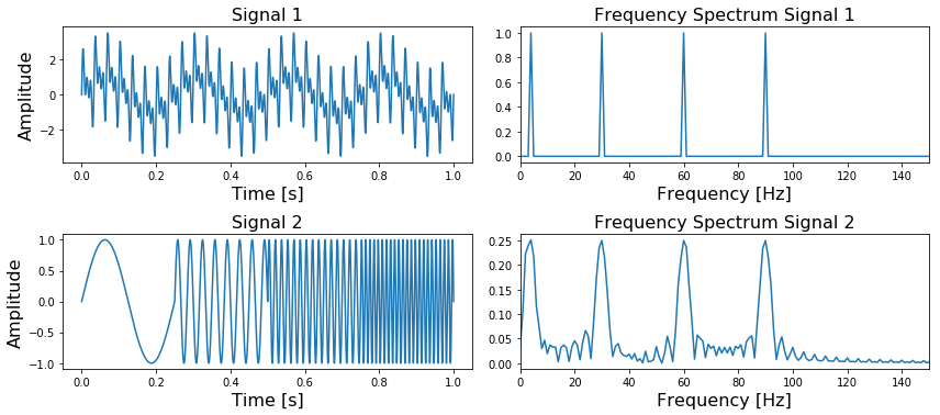
In Figure 1 we can see at the top left a signal containing four different frequencies ( ,
,  ,
,  and
and  ) which are present at all times and on the right its frequency spectrum. In the bottom figure, we can see the same four frequencies, only the first one is present in the first quarter of the signal, the second one in the second quarter, etc. In addition, on the right side we again see its frequency spectrum.
What is important to note here is that the two frequency spectra contain exactly the same four peaks, so it can not tell us where in the signal these frequencies are present. The Fourier Transform can not distinguish between the first two signals.
PS: The side lobes we see in the bottom frequency spectrum, is due to the discontinuity between the four different frequencies.
In trying to overcome this problem, scientists have come up with the Short-Time Fourier Transform. In this approach the original signal is splitted into several parts of equal length (which may or may not have an overlap) by using a sliding window before applying the Fourier Transform. The idea is quite simple: if we split our signal into 10 parts, and the Fourier Transform detects a specific frequency in the second part, then we know for sure that this frequency has occurred between  th and
  th of our original signal.
The main problem with this approach is that you run into the theoretical limits of the Fourier Transform known as the uncertainty principle. The smaller we make the size of the window the more we will know about where a frequency has occurred in the signal, but less about the frequency value itself. The larger we make the size of the window the more we will know about the frequency value and less about the time.
A better approach for analyzing signals with a dynamical frequency spectrum is the Wavelet Transform. The Wavelet Transform has a high resolution in both the frequency- and the time-domain. It does not only tell us which frequencies are present in a signal, but also at which time these frequencies have occurred. This is accomplished by working with different scales. First we look at the signal with a large scale/window and analyze ‘large’ features and then we look at the signal with smaller scales in order to analyze smaller features.
The time- and frequency resolutions of the different methods are illustrated in Figure 2.
In Figure 2 we can see the time and frequency resolutions of the different transformations. The size and orientation of the blocks indicate how small the features are that we can distinguish in the time and frequency domain. The original time-series has a high resolution in the time-domain and zero resolution in the frequency domain. This means that we can distinguish very small features in the time-domain and no features in the frequency domain.
Opposite to that is the Fourier Transform, which has a high resolution in the frequency domain and zero resolution in the time-domain.
The Short Time Fourier Transform has medium sized resolution in both the frequency and time domain.
The Wavelet Transform has:
- for small frequency values a high resolution in the frequency domain, low resolution in the time- domain,
- for large frequency values a low resolution in the frequency domain, high resolution in the time domain.
In other words, the Wavelet Transforms makes a trade-off; at scales in which time-dependent features are interesting it has a high resolution in the time-domain and at scales in which frequency-dependent features are interesting it has a high resolution in the frequency domain.
And as you can imagine, this is exactly the kind of trade-off we are looking for!
2.2 How does the Wavelet Transform work?
The Fourier Transform uses a series of sine-waves with different frequencies to analyze a signal. That is, a signal is represented through a linear combination of sine-waves.
The Wavelet Transform uses a series of functions called wavelets, each with a different scale. The word wavelet means a small wave, and this is exactly what a wavelet is.
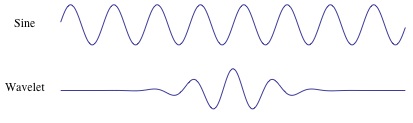
In Figure 3 we can see the difference between a sine-wave and a wavelet. The main difference is that the sine-wave is not localized in time (it stretches out from -infinity to +infinity) while a wavelet is localized in time. This allows the wavelet transform to obtain time-information in addition to frequency information.
Since the Wavelet is localized in time, we can multiply our signal with the wavelet at different locations in time. We start with the beginning of our signal and slowly move the wavelet towards the end of the signal. This procedure is also known as a convolution. After we have done this for the original (mother) wavelet, we can scale it such that it becomes larger and repeat the process. This process is illustrated in the figure below.
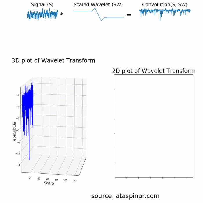
As we can see in the figure above, the Wavelet transform of an 1-dimensional signal will have two dimensions. This 2-dimensional output of the Wavelet transform is the time-scale representation of the signal in the form of a scaleogram.
Above the scaleogram is plotted in a 3D plot in the bottom left figure and in a 2D color plot in the bottom right figure.
PS: You can also have a look at this youtube video to see how a Wavelet Transform works.
So what is this dimension called scale? Since the term frequency is reserved for the Fourier Transform, the wavelet transform is usually expressed in scales instead. That is why the two dimensions of a scaleogram are time and scale. For the ones who find frequencies more intuitive than scales, it is possible to convert scales to pseudo-frequencies with the equation

where  is the pseudo-frequency,
  is the central frequency of the Mother wavelet and
  is the scaling factor.
We can see that a higher scale-factor (longer wavelet) corresponds with a smaller frequency, so by scaling the wavelet in the time-domain we will analyze smaller frequencies (achieve a higher resolution) in the frequency domain. And vice versa, by using a smaller scale we have more detail in the time-domain. So scales are basically the inverse of the frequency.
PS: PyWavelets contains the function scale2frequency to convert from a scale-domain to a frequency-domain.
2.3 The different types of Wavelet families
Another difference between the Fourier Transform and the Wavelet Transform is that there are many different families (types) of wavelets. The wavelet families differ from each other since for each family a different trade-off has been made in how compact and smooth the wavelet looks like. This means that we can choose a specific wavelet family which fits best with the features we are looking for in our signal.
The PyWavelets library for example contains 14 mother Wavelets (families of Wavelets):
Each type of wavelets has a different shape, smoothness and compactness and is useful for a different purpose. Since there are only two mathematical conditions a wavelet has to satisfy it is easy to generate a new type of wavelet.
The two mathematical conditions are the so-called normalization and orthogonalization constraints:
A wavelet must have 1) finite energy and 2) zero mean.
Finite energy means that it is localized in time and frequency; it is integrable and the inner product between the wavelet and the signal always exists.
The admissibility condition implies a wavelet has zero mean in the time-domain, a zero at zero frequency in the time-domain. This is necessary to ensure that it is integrable and the inverse of the wavelet transform can also be calculated.
Furthermore:
- A wavelet can be orthogonal or non-orthogonal.
- A wavelet can be bi-orthogonal or not.
- A wavelet can be symmetric or not.
- A wavelet can be complex or real. If it is complex, it is usually divided into a real part representing the amplitude and an imaginary part representing the phase.
- A wavelets is normalized to have unit energy.
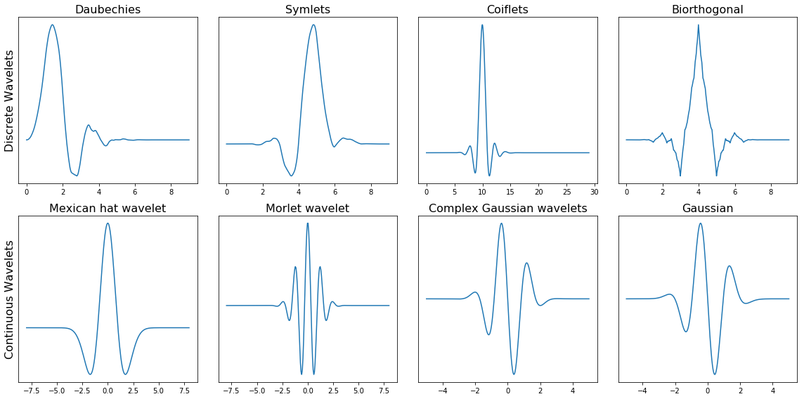
Below we can see a plot with several different families of wavelets.
The first row contains four Discrete Wavelets and the second row four Continuous Wavelets.
PS: To see how all wavelets looks like, you can have a look at the wavelet browser.
Within each wavelet family there can be a lot of different wavelet subcategories belonging to that family. You can distinguish the different subcategories of wavelets by the number of coefficients (the number of vanishing moments) and the level of decomposition.
This is illustrated below in for the one family of wavelets called ‘Daubechies’.

In Figure 6 we can see wavelets of the ‘Daubechies’ family (db) of wavelets. In the first column we can see the Daubechies wavelets of the first order ( db1), in the second column of the second order (db2), up to the fifth order in the fifth column. PyWavelets contains Daubechies wavelets up to order 20 (db20).
The number of the order indicates the number of vanishing moments. So db3 has three vanishing moments and db5 has 5 vanishing moment. The number of vanishing moments is related to the approximation order and smoothness of the wavelet. If a wavelet has p vanishing moments, it can approximate polynomials of degree p – 1.
When selecting a wavelet, we can also indicate what the level of decomposition has to be. By default, PyWavelets chooses the maximum level of decomposition possible for the input signal. The maximum level of decomposition (see pywt.dwt_max_level()) depends on the length of the input signal length and the wavelet (more on this later).
As we can see, as the number of vanishing moments increases, the polynomial degree of the wavelet increases and it becomes smoother. And as the level of decomposition increases, the number of samples this wavelet is expressed in increases.
2.4 Continuous Wavelet Transform vs Discrete Wavelet Transform
As we have seen before (Figure 5), the Wavelet Transform comes in two different and distinct flavors; the Continuous and the Discrete Wavelet Transform.
Mathematically, a Continuous Wavelet Transform is described by the following equation:
![]()
where  is the continuous mother wavelet which gets scaled by a factor of and translated by a factor of
  . The values of the scaling and translation factors are continuous, which means that there can be an infinite amount of wavelets. You can scale the mother wavelet with a factor of 1.3, or 1.31, and 1.311, and 1.3111 etc.
When we are talking about the Discrete Wavelet Transform, the main difference is that the DWT uses discrete values for the scale and translation factor. The scale factor increases in powers of two, so  and the translation factor increases integer values (
  ).
).
PS: The DWT is only discrete in the scale and translation domain, not in the time-domain. To be able to work with digital and discrete signals we also need to discretize our wavelet transforms in the time-domain. These forms of the wavelet transform are called the Discrete-Time Wavelet Transform and the Discrete-Time Continuous Wavelet Transform.
2.5 More on the Discrete Wavelet Transform: The DWT as a filter-bank.
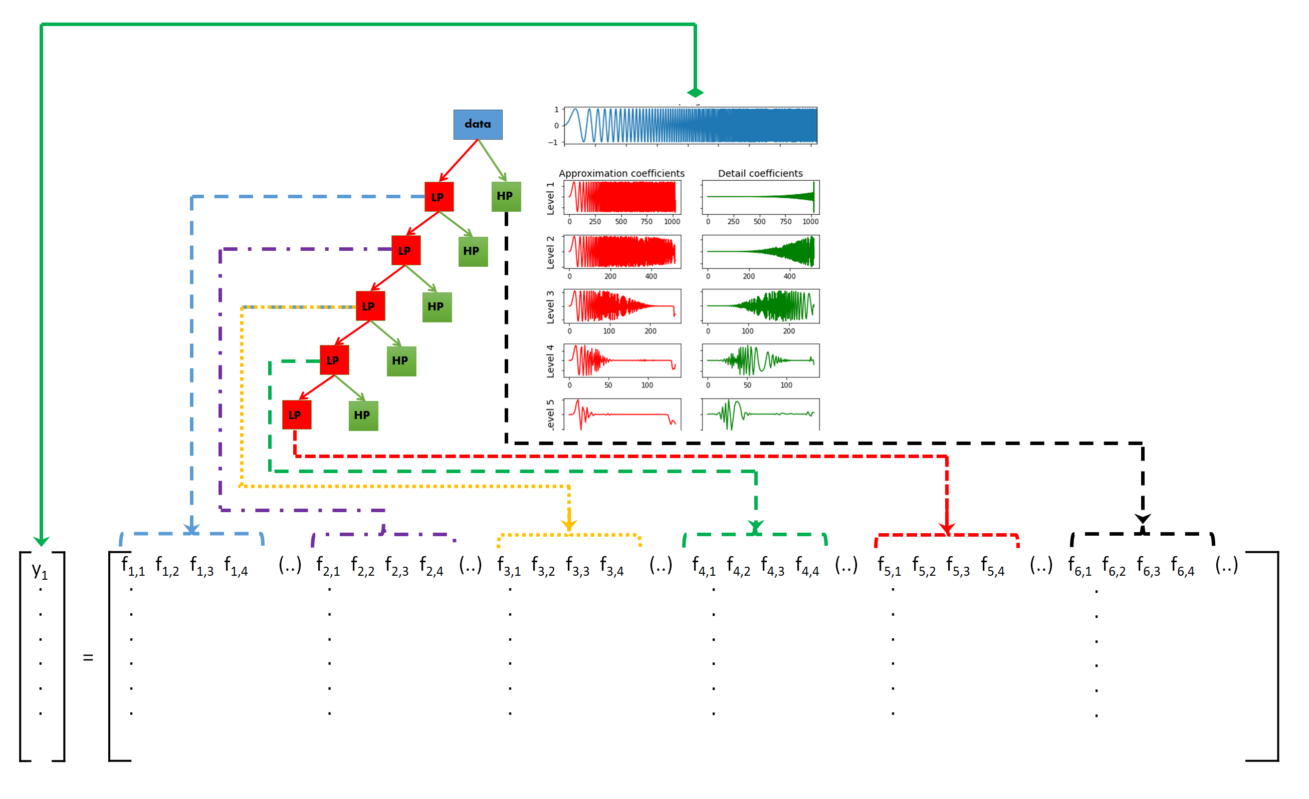
In practice, the DWT is always implemented as a filter-bank. This means that it is implemented as a cascade of high-pass and low-pass filters. This is because filter banks are a very efficient way of splitting a signal of into several frequency sub-bands.
Below I will try to explain the concept behind the filter-bank in a simple (and probably oversimplified) way. It is necessary in order to understand how the wavelet transform actually works and can be used in practical applications.
To apply the DWT on a signal, we start with the smallest scale. As we have seen before, small scales correspond with high frequencies. This means that we first analyze high frequency behavior. At the second stage, the scale increases with a factor of two (the frequency decreases with a factor of two), and we are analyzing behavior around half of the maximum frequency. At the third stage, the scale factor is four and we are analyzing frequency behavior around a quarter of the maximum frequency. And this goes on and on, until we have reached the maximum decomposition level.
What do we mean with maximum decomposition level? To understand this we should also know that at each subsequent stage the number of samples in the signal is reduced with a factor of two. At lower frequency values, you will need less samples to satisfy the Nyquist rate so there is no need to keep the higher number of samples in the signal; it will only cause the transform to be computationally expensive. Due to this downsampling, at some stage in the process the number of samples in our signal will become smaller than the length of the wavelet filter and we will have reached the maximum decomposition level.
To give an example, suppose we have a signal with frequencies up to 1000 Hz. In the first stage we split our signal into a low-frequency part and a high-frequency part, i.e. 0-500 Hz and 500-1000 Hz.
At the second stage we take the low-frequency part and again split it into two parts: 0-250 Hz and 250-500 Hz.
At the third stage we split the 0-250 Hz part into a 0-125 Hz part and a 125-250 Hz part.
This goes on until we have reached the level of refinement we need or until we run out of samples.
We can easily visualize this idea, by plotting what happens when we apply the DWT on a chirp signal. A chirp signal is a signal with a dynamic frequency spectrum; the frequency spectrum increases with time. The start of the signal contains low frequency values and the end of the signal contains the high frequencies. This makes it easy for us to visualize which part of the frequency spectrum is filtered out by simply looking at the time-axis.

In Figure 7 we can see our chirp signal, and the DWT applied to it subsequently. There are a few things to notice here:
- In PyWavelets the DWT is applied with
pywt.dwt() - The DWT return two sets of coefficients; the approximation coefficients and detail coefficients.
- The approximation coefficients represent the output of the low pass filter (averaging filter) of the DWT.
- The detail coefficients represent the output of the high pass filter (difference filter) of the DWT.
- By applying the DWT again on the approximation coefficients of the previous DWT, we get the wavelet transform of the next level.
- At each next level, the original signal is also sampled down by a factor of 2.
So now we have seen what it means that the DWT is implemented as a filter bank; At each subsequent level, the approximation coefficients are divided into a coarser low pass and high pass part and the DWT is applied again on the low-pass part.
As we can see, our original signal is now converted to several signals each corresponding to different frequency bands. Later on we will see how the approximation and detail coefficients at the different frequency sub-bands can be used in applications like removing high frequency noise from signals, compressing signals, or classifying the different types signals.
PS: We can also use pywt.wavedec() to immediately calculate the coefficients of a higher level. This functions takes as input the original signal and the level  and returns the one set of approximation coefficients (of the n-th level) and n sets of detail coefficients (1 to n-th level).
PS2: This idea of analyzing the signal on different scales is also known as multiresolution / multiscale analysis, and decomposing your signal in such a way is also known as multiresolution decomposition, or sub-band coding.
3.1 Visualizing the State-Space using the Continuous Wavelet Transform
So far we have seen what the wavelet transform is, how it is different from the Fourier Transform, what the difference is between the CWT and the DWT, what types of wavelet families there are, what the impact of the order and level of decomposition is on the mother wavelet, and how and why the DWT is implemented as a filter-bank.
We have also seen that the output of a wavelet transform on a 1D signal results in a 2D scaleogram. Such a scaleogram gives us detailed information about the state-space of the system, i.e. it gives us information about the dynamic behavior of the system.
The el-Nino dataset is a time-series dataset used for tracking the El Nino and contains quarterly measurements of the sea surface temperature from 1871 up to 1997. In order to understand the power of a scaleogram, let us visualize it for el-Nino dataset together with the original time-series data and its Fourier Transform.
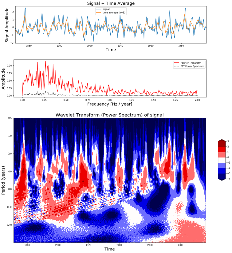
In Figure 8 we can see in the top figure the el-Nino dataset together with its time average, in the middle figure the Fourier Transform and at the bottom figure the scaleogram produced by the Continuous Wavelet Transform.
In the scaleogram we can see that most of the power is concentrated in a 2-8 year period. If we convert this to frequency (T = 1 / f) this corresponds with a frequency of 0.125 – 0.5 Hz. The increase in power can also be seen in the Fourier transform around these frequency values. The main difference is that the wavelet transform also gives us temporal information and the Fourier Transform does not. For example, in the scaleogram we can see that up to 1920 there were many fluctuations, while there were not so much between 1960 – 1990. We can also see that there is a shift from shorter to longer periods as time progresses. This is the kind of dynamic behavior in the signal which can be visualized with the Wavelet Transform but not with the Fourier Transform.
This should already make clear how powerful the wavelet transform can be for machine learning purposes. But to make the story complete, let us also look at how this can be used in combination with a Convolutional Neural Network to classify signals.
3.2 Using the Continuous Wavelet Transform and a Convolutional Neural Network for classification of signals
In section 3.1 we have seen that the wavelet transform of a 1D signal results in a 2D scaleogram which contains a lot more information than just the time-series or just the Fourier Transform. We have seen that applied on the el-Nino dataset, it can not only tell us what the period is of the largest oscillations, but also when these oscillations were present and when not.
Such a scaleogram can not only be used to better understand the dynamical behavior of a system, but it can also be used to distinguish different types of signals produced by a system from each other.
If you record a signal while you are walking up the stairs or down the stairs, the scaleograms will look different. ECG measurements of people with a healthy heart will have different scaleograms than ECG measurements of people with arrhythmia. Or measurements on a bearing, motor, rotor, ventilator, etc when it is faulty vs when it not faulty. The possibilities are limitless!
So by looking at the scaleograms we can distinguish a broken motor from a working one, a healthy person from a sick one, a person walking up the stairs from a person walking down the stairs, etc etc. But if you are as lazy as me, you probably don’t want to sift through thousands of scaleograms manually. One way to automate this process is to build a Convolutional Neural Network which can automatically detect the class each scaleogram belongs to and classify them accordingly.
What was the deal again with CNN? In previous blog posts we have seen how we can use Tensorflow to build a convolutional neural network from scratch. And how we can use such a CNN to detect roads in satellite images. If you are not familiar with CNN’s it is a good idea to have a look at these previous blog posts, since the rest of this section assumes you have some knowledge of CNN’s.
In the next few sections we will load a dataset (containing measurement of people doing six different activities), visualize the scaleograms using the CWT and then use a Convolutional Neural Network to classify these scaleograms.
3.2.1. Loading the UCI-HAR time-series dataset
Let us try to classify an open dataset containing time-series using the scaleograms and a CNN. The Human Activity Recognition Dataset (UCI-HAR) contains sensor measurements of people while they were doing different types of activities, like walking up or down the stairs, laying, standing, walking, etc. There are in total more than 10.000 signals where each signal consists of nine components (x acceleration, y acceleration, z acceleration, x,y,z gyroscope, etc). This is the perfect dataset for us to try our use case of CWT + CNN!
PS: For more on how the UCI HAR dataset looks like, you can also have a look at the previous blog post in which it was described in more detail.
After we have downloaded the data, we can load it into a numpy nd-array in the following way:
The training set contains 7352 signals where each signal has 128 measurement samples and 9 components. The signals from the training set are loaded into a numpy ndarray of size (7352 , 128, 9) and the signals from the test set into one of size (2947 , 128, 9).
Since the signal consists of nine components we have to apply the CWT nine times for each signal. Below we can see the result of the CWT applied on two different signals from the dataset. The left one consist of a signal measured while walking up the stairs and the right one is a signal measured while laying down.
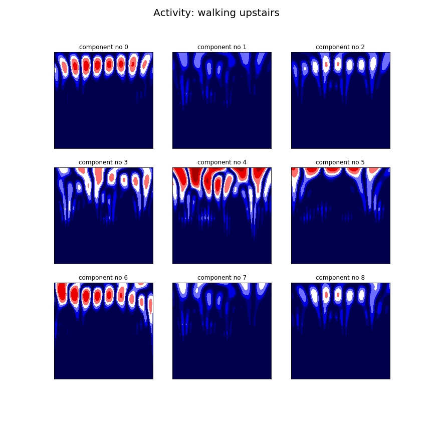
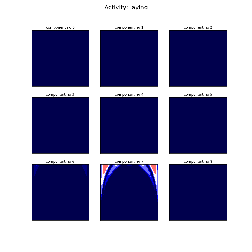
Figure 9. The CWT applied on two signals belonging to the UCI HAR dataset. Each signal has nine different components. On the left we can see the signals measured during walking upstairs and on the right we can see a signal measured during laying.
3.2.2 Applying the CWT on the dataset and transforming the data to the right format
Since each signal has nine components, each signal will also have nine scaleograms. So the next question to ask is, how do we feed this set of nine scaleograms into a Convolutional Neural Network? There are several options we could follow:
- Train a CNN for each component separately and combine the results of the nine CNN’s in some sort of an ensembling method. I suspect that this will generally result in a poorer performance since the inter dependencies between the different components are not taken into account.
- Concatenate the nine different signals into one long signal and apply the CWT on the concatenated signal. This could work but there will be discontinuities at location where two signals are concatenated and this will introduced noise in the scaleogram at the boundary locations of the component signals.
- Calculate the CWT first and thén concatenate the nine different CWT images into one and feed that into the CNN. This could also work, but here there will also be discontinuities at the boundaries of the CWT images which will feed noise into the CNN. If the CNN is deep enough, it will be able to distinguish between these noisy parts and actually useful parts of the image and choose to ignore the noise. But I still prefer option number four:
- Place the nine scaleograms on top of each other and create one single image with nine channels. What does this mean? Well, normally an image has either one channel (grayscale image) or three channels (color image), but our CNN can just as easily handle images with nine channels. The way the CNN works remains exactly the same, the only difference is that there will be three times more filters compared to an RGB image.
This process is illustrated in the Figure 11.

Below we can see the Python code on how to apply the CWT on the signals in the dataset, and reformat it in such a way that it can be used as input for our Convolutional Neural Network. The total dataset contains over 10.000 signals, but we will only use 5.000 signals in our training set and 500 signals in our test set.
As you can see above, the CWT of a single signal-component (128 samples) results in an image of 127 by 127 pixels. So the scaleograms coming from the 5000 signals of the training dataset are stored in an numpy ndarray of size (5000, 127, 127, 9) and the scaleograms coming from the 500 test signals are stored in one of size (500, 127, 127, 9).
3.2.3 Training the Convolutional Neural Network with the CWT
Now that we have the data in the right format, we can start with the most interesting part of this section: training the CNN! For this part you will need the keras library, so please install it first.
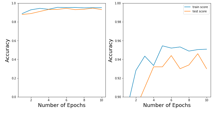
As you can see, combining the Wavelet Transform and a Convolutional Neural Network leads to an awesome and amazing result!
We have an accuracy of 94% on the Activity Recognition dataset. Much higher than you can achieve with any other method.
In section 3.5 we will use the Discrete Wavelet Transform instead of Continuous Wavelet Transform to classify the same dataset and achieve similarly amazing results!
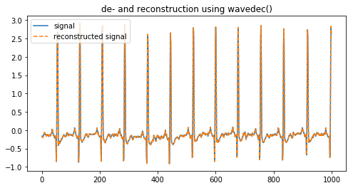
3.3 Deconstructing a signal using the DWT
In Section 2.5 we have seen how the DWT is implemented as a filter-bank which can deconstruct a signal into its frequency sub-bands. In this section, let us see how we can use PyWavelets to deconstruct a signal into its frequency sub-bands and reconstruct the original signal again.
PyWavelets offers two different ways to deconstruct a signal.
- We can either apply
pywt.dwt()on a signal to retrieve the approximation coefficients. Then apply the DWT on the retrieved coefficients to get the second level coefficients and continue this process until you have reached the desired decomposition level. - Or we can apply
pywt.wavedec()directly and retrieve all of the the detail coefficients up to some level. This functions takes as input the original signal and the level and returns the one set of approximation coefficients (of the n-th level) and n sets of detail coefficients (1 to n-th level).
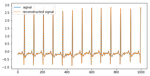
Above we have deconstructed a signal into its coefficients and reconstructed it again using the inverse DWT.
The second way is to use pywt.wavedec() to deconstruct and reconstruct a signal and it is probably the most simple way if you want to get higher-level coefficients.
3.4 Removing (high-frequency) noise using the DWT
In the previous section we have seen how we can deconstruct a signal into the approximation (low pass) and detail (high pass) coefficients. If we reconstruct the signal using these coefficients we will get the original signal back.
But what happens if we reconstruct while we leave out some detail coefficients? Since the detail coefficients represent the high frequency part of the signal, we will simply have filtered out that part of the frequency spectrum. If you have a lot of high-frequency noise in your signal, this one way to filter it out.
Leaving out of the detail coefficients can be done using pywt.threshold(), which removes coefficient values higher than the given threshold.
Lets demonstrate this using NASA’s Femto Bearing Dataset. This is a dataset containing high frequency sensor data regarding accelerated degradation of bearings.
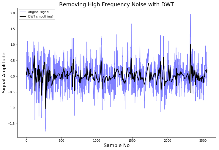
As we can see, by deconstructing the signal, setting some of the coefficients to zero, and reconstructing it again, we can remove high frequency noise from the signal.
People who are familiar with signal processing techniques might know there are a lot of different ways to remove noise from a signal. For example, the Scipy library contains a lot of smoothing filters (one of them is the famous Savitzky-Golay filter) and they are much simpler to use. Another method for smoothing a signal is to average it over its time-axis.
So why should you use the DWT instead? The advantage of the DWT again comes from the many wavelet shapes there are available. You can choose a wavelet which will have a shape characteristic to the phenomena you expect to see. In this way, less of the phenomena you expect to see will be smoothed out.
3.5 Using the Discrete Wavelet Transform to classify signals
In Section 3.2 we have seen how we can use a the CWT and a CNN to classify signals. Of course it is also possible to use the DWT to classify signals. Let us have a look at how this could be done.
3.5.1 The idea behind Discrete Wavelet classification
The idea behind DWT signal classification is as follows: The DWT is used to split a signal into different frequency sub-bands, as many as needed or as many as possible. If the different types of signals exhibit different frequency characteristics, this difference in behavior has to be exhibited in one of the frequency sub-bands. So if we generate features from each of the sub-band and use the collection of features as an input for a classifier (Random Forest, Gradient Boosting, Logistic Regression, etc) and train it by using these features, the classifier should be able to distinguish between the different types of signals.
This is illustrated in the figure below:
3.5.2 Generating features per sub-band
So what kind of features can be generated from the set of values for each of the sub-bands? Of course this will highly depend on the type of signal and the application. But in general, below are some features which are most frequently used for signals.
- Auto-regressive model coefficient values
- (Shannon) Entropy values; entropy values can be taken as a measure of complexity of the signal.
- Statistical features like:
- variance
- standard deviation
- Mean
- Median
- 25th percentile value
- 75th percentile value
- Root Mean Square value; square of the average of the squared amplitude values
- The mean of the derivative
- Zero crossing rate, i.e. the number of times a signal crosses y = 0
- Mean crossing rate, i.e. the number of times a signal crosses y = mean(y)
These are just some ideas you could use to generate the features out of each sub-band. You could use some of the features described here, or you could use all of them. Most classifiers in the scikit-learn package are powerful enough to handle a large number of input features and distinguish between useful ones and non-useful ones. However, I still recommend you think carefully about which feature would be useful for the type of signal you are trying to classify.
PS: There are a hell of a lot more statistical functions in scipy.stats. By using these you can create more features if necessary.
Let’s see how this could be done in Python for a few of the above mentioned features:
Above we can see
- a function to calculate the entropy value of an input signal,
- a function to calculate some statistics like several percentiles, mean, standard deviation, variance, etc,
- a function to calculate the zero crossings rate and the mean crossings rate,
- and a function to combine the results of these three functions.
The final function returns a set of 12 features for any list of values. So if one signal is decomposed into 10 different sub-bands, and we generate features for each sub-band, we will end up with 10*12 = 120 features per signal.
3.5.3 Using the features and scikit-learn classifiers to classify two ECG datasets.
So far so good. The next step is to actually use the DWT to decompose the signals in the training set into its sub-bands, calculate the features for each sub-band, use the features to train a classifier and use the classifier to predict the signals in the test-set.
We will do this for two time-series datasets:
- The UCI-HAR dataset which we have already seen in section 3.2. This dataset contains smartphone sensor data of humans while doing different types of activities, like sitting, standing, walking, stair up and stair down.
- PhysioNet ECG Dataset (download from here) which contains a set of ECG measurements of healthy persons (indicated as Normal sinus rhythm, NSR) and persons with either an arrhythmia (ARR) or a congestive heart failure (CHF). This dataset contains 96 ARR measurements, 36 NSR measurements and 30 CHF measurements.
After we have downloaded both datasets, and placed them in the right folders, the next step is to load them into memory. We have already seen how we can load the UCI-HAR dataset in section 3.2, and below we can see how to load the ECG dataset.
The ECG dataset is saved as a MATLAB file, so we have to use scipy.io.loadmat() to open this file in Python and retrieve its contents (the ECG measurements and the labels) as two separate lists.
The UCI HAR dataset is saved in a lot of .txt files, and after reading the data we save it into an numpy ndarray of size (no of signals, length of signal, no of components) = (10299 , 128, 9)
Now let us have a look at how we can get features out of these two datasets.
What we have done above is to write functions to generate features from the ECG signals and the UCI HAR signals. There is nothing special about these functions and the only reason we are using two seperate functions is because the two datasets are saved in different formats. The ECG dataset is saved in a list, and the UCI HAR dataset is saved in a 3D numpy ndarray.
For the ECG dataset we iterate over the list of signals, and for each signal apply the DWT which returns a list of coefficients. For each of these coefficients, i.e. for each of the frequency sub-bands, we calculate the features with the function we have defined previously. The features calculated from all of the different coefficients belonging to one signal are concatenated together, since they belong to the same signal.
The same is done for the UCI HAR dataset. The only difference is that we now have two for-loops since each signal consists of nine components. The features generated from each of the sub-band from each of the signal component are concatenated together.
Now that we have calculated the features for the two datasets, we can use a GradientBoostingClassifier from the scikit-learn library and train it.
PS: If you want to know more about classification with the scikit-learn library, you can have a look at this blog post.
As we can see, the results when we use the DWT + Gradient Boosting Classifier are equally amazing!
This approach has an accuracy on the UCI-HAR test set of 95% and an accuracy on the ECG test set of 93%.
3.6 Comparison of the classification accuracies between DWT, Fourier Transform and Recurrent Neural Networks
So far, we have seen throughout the various blog-posts, how we can classify time-series and signals in different ways. In a previous post we have classified the UCI-HAR dataset using Signal Processing techniques like The Fourier Transform. The accuracy on the test-set was ~91%.
In another blog-post, we have classified the same UCI-HAR dataset using Recurrent Neural Networks. The highest achieved accuracy on the test-set was ~86%.
In this blog-post we have achieved an accuracy of ~94% on the test-set with the approach of CWT + CNN and an accuracy of ~95% with the DWT + GradientBoosting approach!
It is clear that the Wavelet Transform has far better results. We could repeat this for other datasets and I suspect there the Wavelet Transform will also outperform.
What we can also notice is that strangely enough Recurrent Neural Networks perform the worst. Even the approach of simply using the Fourier Transform and then the peaks in the frequency spectrum has an better accuracy than RNN’s.
This really makes me wonder, what the hell Recurrent Neural Networks are actually good for. It is said that a RNN can learn ‘temporal dependencies in sequential data’. But, if a Fourier Transform can fully describe any signal (no matter its complexity) in terms of the Fourier components, then what more can be learned with respect to ‘temporal dependencies’.
It is no wonder that people already start talking about the fall of RNN / LSTM.
PS: The achieved accuracy using the DWT will depend on the features you decide to calculate, the wavelet and the classifier you decide to use. To give an impression, below are the accuracy values for the test set of the UCI-HAR and ECG datasets, for all of the wavelets present in PyWavelets, and for the most used 5 classifiers in scikit-learn.

We can see that there will be differences in accuracy depending on the chosen classifier. Generally speaking, the Gradient Boosting classifier performs best. This should come as no surprise since almost all kaggle competitions are won with the gradient boosting model.
What is more important is that the chosen wavelet can also have a lot of influence on the achieved accuracy values. Unfortunately I do not have an guideline on choosing the right wavelet. The best way to choose the right wavelet is to do a lot of trial-and-error and a little bit of literature research.
4. Final Words
In this blog post we have seen how we can use the Wavelet Transform for the analysis and classification of time-series and signals (and some other stuff). Not many people know how to use the Wavelet Transform, but this is mostly because the theory is not beginner-friendly and the wavelet transform is not readily available in open source programming languages.
MATLAB is one the few programming languages with a very complete Wavelet Toolbox. But since MATLAB has a expensive licensing fee, it is mostly used in the academic world and large corporations.
Among Data Scientists, the Wavelet Transform remains an undiscovered jewel and I recommend fellow Data Scientists to use it more often. I am very thankful to the contributors of the PyWavelets package who have implemented a large set of Wavelet families and higher level functions for using these wavelets. Thanks to them, Wavelets can now more easily be used by people using the Python programming language.
I have tried to give a concise but complete description of how wavelets can be used for the analysis of signals. I hope it has motivated you to use it more often and that the Python code provided in this blog-post will point you in the right direction in your quest to use wavelets for data analysis.
A lot will depend on the choices you make; which wavelet transform will you use, CWT or DWT? which wavelet family will you use? Up to which level of decomposition will you go? What is the right range of scales to use?
Like most things in life, the only way to master a new method is by a lot of practice. You can look up some literature to see what the commonly used wavelet type is for your specific problem, but do not make the mistake of thinking whatever you read in research papers is the holy and you don’t need to look any further. 
PS: You can also find the code in this blog-post in five different Jupyter notebooks in my Github repository.
No hay comentarios:
Publicar un comentario