http://math.jacobs-university.de/oliver/teaching/iub/resources/octave/octave-intro/octave-intro.html
Introduction to GNU Octave
Hubert Selhofer, revised by Marcel Oliver
updated to current Octave version by Thomas L. Scofield
Date: 2008/08/16
![\includegraphics[height=10cm]{sombr}](http://math.jacobs-university.de/oliver/teaching/iub/resources/octave/octave-intro/img1.png)
Contents
- 1 Basics
- 2 Vector and matrix operations
- 2.1 Vectors
- 2.2 Matrices
- 2.3 Basic matrix arithmetic
- 2.4 Element-wise operations
- 2.5 Indexing and slicing
- 2.6 Solving linear systems of equations
- 2.7 Inverses, decompositions, eigenvalues
- 2.8 Testing for zero elements
- 3 Control structures
- 3.1 Functions
- 3.2 Global variables
- 3.3 Loops
- 3.4 Branching
- 3.5 Functions of functions
- 3.6 Efficiency considerations
- 3.7 Input and output
- 4 Graphics
- 5 Exercises
1 Basics
1.1 What is Octave?
Octave is an interactive programming language specifically suited for vectorizable numerical calculations. It provides a high level interface to many standard libraries of numerical mathematics, e.g. LAPACK or BLAS.
The syntax of Octave resembles that of Matlab. An Octave program usually runs unmodified on Matlab. Matlab, being commercial software, has a larger function set, and so the reverse does not always work, especially when the program makes use of specialized add-on toolboxes for Matlab.
1.2 Help!
- help lists the names of all built-in functions and internal variables.
- help name further explains the variable or function ``name''.
Example:
octave:1> help eig
1.3 Input conventions
- All commands can be typed in at the prompt or read from a script.
- Scripts are plain text files with file suffix .m. They are imported by calling the file name without the suffix and behave as if their content was typed in line by line.
- ; separates several commands within a line. A command terminated by ; does not display its result on-screen.
- , separates two commands without suppressing on-screen output.
- ... at the end of the line denotes that an expression continues into the next line.
- Comments are preceded by %.
- Octave is case sensitive.
1.4 Variables and standard operations
- varname = expression assigns the result of expression to varname.
- Octave has all the usual mathematical functions +, -, *, /, ^, sin, cos, exp, acos, abs, etc.
- The operators of elementary logic are:
< smaller <= smaller or equal & and > greater >= greater or equal | or == equal ~=not equal ~not
When debugging user-defined objects, the following commands are useful:
- whos shows all user-defined variables and functions (see Section 3.1).
- clear name clears name from memory; if no name is given, all variables and functions will be cleared.
- type name displays information about the variable or function name on the screen.
Examples:
  octave:1> x12 = 1/8, long_name = 'A String'
  x12 = 0.12500
  long_name = A String
  octave:2> sqrt(-1)-i
  ans = 0
  octave:3> x = sqrt(2); sin(x)/x
  ans = 0.69846
And here is a script doless, saved in a file named doless.m:
  one = 1;
  two = 2;
  three = one + two;
Calling the script:
  octave:1> doless
  octave:2> whos
  *** local user variables:
  prot  type               rows   cols  name
  ====  ====               ====   ====  ====
   wd   real scalar           1      1  three
   wd   real scalar           1      1  one
   wd   real scalar           1      1  two
2 Vector and matrix operations
Matrices and vectors are the most important building blocks for programming in Octave.
2.1 Vectors
- Row vector:
 :
:v = [ 1 2 3 ]
- Column vector:
 :
:v = [ 1; 2; 3 ]
- Automatic generation of vectors with constant increment:
Start[:Increment]:End
Examples:
  octave:1> x = 3:6
  x =
    3  4  5  6
  octave:2> y = 0:.15:.7
  y =
  0.00000  0.15000  0.30000  0.45000  0.60000
  octave:3> z = pi:-pi/4:0
  z =
  3.14159  2.35619  1.57080  0.78540  0.00000
2.2 Matrices
A matrix  is generated as follows.
  octave:1> A = [ 1 2; 3 4]
  A =
    1  2
    3  4
Matrices can assembled from submatrices:
  octave:2> b = [5; 6];
  octave:3> M = [A b]
  M =

    1  2  5
    3  4  6
There are functions to create frequently used ![]() matrices. If
matrices. If ![]() , only one argument is necessary.
, only one argument is necessary.
- eye(m,n) produces a matrix with ones on the main diagonal and zeros elsewhere. When
 , the identity matrix is generated.
 - zeros(m,n) generates the zero matrix of dimension
 .
. - ones(m,n) generates an matrix where all entries are
 .
. - rand(m,n) generates a random matrix whose entries are uniformly distributed in the interval
 .
.
2.3 Basic matrix arithmetic
- +, -, and * denote matrix addition, subtraction, and multiplication.
- A' transposes and conjugates A.
- A.' transposes A.
Examples:
  octave:1> A = [1 2; 3 4]; B = 2*ones(2,2);
  octave:2> A+B, A-B, A*B
  ans =
    3  4
    5  6
  ans =
    -1   0
     1   2
  ans =
     6   6
    14  14
2.4 Element-wise operations
While * refers to the usual matrix multiplication, .* denotes element-wise multiplication. Similarly, ./ and .^ denote the element-wise division and power operators.
Examples:
  octave:1> A = [1 2; 3 4]; A.^2   % Element-wise power
  ans =

     1   4
     9  16

  octave:2> A^2   % Proper matrix power: A^2 = A*A
  ans =

     7  10
    15  22
2.5 Indexing and slicing
- v(k) is the
 -th element of the row or column vector
  .
. - A(k,l) is the matrix element
 .
. - v(m:n) is the ``slice'' of the vector from its
 th to its
  -th entry.
 - A(k,:) is the th row of matrix
 .
. - A(:,l) is the
 th column of matrix .
Querying dimensions:
- length(v) returns the number of elements of the vector .
- [Rows,Columns] = size(A) returns the number of rows and columns of the matrix .
Reshaping:
- reshape(A,m,n) transforms A into an -matrix.
- diag(A) creates a column vector containing the diagonal elements
 of the matrix A.
 - diag(v) generates a matrix with the elements from the vector v on the diagonal.
- diag(v,k) generates a matrix with the elements from the vector v on the k-th diagonal.
- A(k,:) = rv assigns to the k-th row of A the row vector rv.
- A(k,:) = [] deletes the k-th row of A.
- A(:,j) = cv assigns to the j-th column of A the column vector cv.
- A(:,j) = [] deletes the j-th column of A.
Examples:
  octave:1> A = [1 2 3; 4 5 6]; v = [7; 8];
  octave:2> A(2,3) = v(2)
  A =

    1  2  3
    4  5  8

  octave:3> A(:,2) = v
  A =

    1  7  3
    4  8  8

  octave:4> A(1,1:2) = v'
  A =

    7  8  3
    4  8  8
2.6 Solving linear systems of equations
A\bsolves the equation .
.
2.7 Inverses, decompositions, eigenvalues
- B = inv(A) computes the inverse of .
- [L,U,P] = lu(A) computes the LU-decomposition
 .
. - [Q,R] = qr(A) computes the QR-decomposition
 .
. - R = chol(A) computes the Cholesky decomposition of .
- S = svd(A) computes the singular values of .
- H = hess(A) brings into Hessenberg form.
- E = eig(A) computes the eigenvalues of .
- [V,D] = eig(A) computes a diagonal matrix
 , containing the eigenvalues of , and a matrix
  containing the corresponding eigenvectors such that
  .
. - norm(X,p) calculates the
 -norm of vector
  . If is a matrix, can only take the values 1, 2 or inf. The default is
  .
. - cond(A) computes the condition number of with respect to the
 -norm.
A lot of these commands support further options. They can be listed by typing help funcname.
2.8 Testing for zero elements
- [i,j,v] = find(A) finds the indices of all nonzero elements of A. The resulting vectors satisfy
 .
. - any(v) returns if the vector v contains nonzero elements.
- any(A) applies any to each of the columns of the matrix A.
3 Control structures
3.1 Functions
Traditionally, functions are also stored in plain text files with suffix .m. In contrast to scripts, functions can be called with arguments, and all variables used within the function are local--they do not influence variables defined previously.
Example:
A function f, saved in the file named f.m.
  function y = f (x)
    y = cos(x/2)+x;
  end
Remark:
In Octave, several functions can be defined in a single script file. Matlab on the other hand, strictly enforces one function per .m file, where the name of the function must match the name of the file. If compatibility with Matlab is important, this restriction should also be applied to programs written in Octave.
Example with two function values:
A function dolittle, which is saved in the file named dolittle.m.
  function [out1,out2] = dolittle (x)
    out1 = x^2;
    out2 = out1*x;
  end
Calling the function:
  octave:1> [x1,x2]=dolittle(2)
  x1 = 4
  x2 = 8
  octave:2> whos
  *** currently compiled functions:
  prot  type               rows   cols  name
  ====  ====               ====   ====  ====
   wd   user function         -      -  dolittle
  *** local user variables:
  prot  type               rows   cols  name
  ====  ====               ====   ====  ====
   wd   real scalar           1      1  x1
   wd   real scalar           1      1  x2
Obviously, the variables out1 and out2 were local to dolittle. Previously defined variables out1 or out2 would not have been affected by calling dolittle.
3.2 Global variables
global name declares name as a global variable.
Example:
A function foo in the file named foo.m:
  global N   % makes N a global variable; may be set in main file

  function out = foo(arg1,arg2)
  global N   % makes local N refer to the global N
  <Computation>
  end
If you change N within the function, it changes in the value of N everywhere.
3.3 Loops
The syntax of for- and while-loops is immediate from the following examples:
  for n = 1:10
    [x(n),y(n)]=dolittle(n);
  end

  while t<T
    t = t+h;
  end
For-loop backward:
  for n = 10:-1:1
  ...
3.4 Branching
Conditional branching works as follows.
  if x==0
    error('x is 0!');
  else
    y = 1/x;
  end

  switch pnorm
    case 1
      sum(abs(v))
    case inf
      max(abs(v))
    otherwise
      sqrt(v'*v)
  end
3.5 Functions of functions
- eval(string) evaluates string as Octave code.
- feval(funcname,arg1,
 ) is equivalent to calling funcname with arguments arg1, .
Example:
Approximate an integral by the midpoint rule:
We define two functions, gauss.m and mpr.m, as follows:
  function y = gauss(x)
    y = exp(-x.^2/2);
  end

  function S = mpr(fun,a,b,N)
    h = (b-a)/N;
    S = h*sum(feval(fun,[a+h/2:h:b]));
  end
Now the function gauss can be integrated by calling:
octave:1> mpr('gauss',0,5,500)
3.6 Efficiency considerations
Loops and function calls, especially through feval, have a very high computational overhead. Therefore, if possible, vectorize all operations.
Example:
We are programming the midpoint rule from the previous section with a for-loop (file name is mpr_long.m):
  function S = mpr_long(fun,a,b,N)
    h = (b-a)/N; S = 0;
    for k = 0:(N-1),
      S = S + feval(fun,a+h*(k+1/2));
    end
    S = h*S;
  end
We verify that mpr and mpr_long yield the same answer, and compare the evaluation times.
  octave:1> t = cputime;
  > Int1=mpr('gauss',0,5,500); t1=cputime-t;
  octave:2> t = cputime;
  > Int2=mpr_long('gauss',0,5,500); t2=cputime-t;
  octave:3> Int1-Int2, t2/t1
  ans = 0
  ans = 45.250
3.7 Input and output
- save data var1 [var2 ] saves the values of variables var1 etc. into the file data.
- load data reads the file data, restoring the values of the previously saved variables.
- fprintf(string[,var1, ]) resembles C syntax for formatting output, see man fprintf under Unix.
- format [long|short] enlarges or reduces the number of decimals displayed. Calling format without argument restores the default.
- pause Suspends evaluation until a key is pressed.
Example:
  octave:1> for k = .1:.2:.5,
  > fprintf('1/%g = %10.2e\n',k,1/k); end
  1/0.1 =   1.00e+01
  1/0.3 =   3.33e+00
  1/0.5 =   2.00e+00
4 Graphics
4.1 2D graphics
- plot(x,y[,fmt]) plots a line through the points
 . With the string fmt you can select line style and color; see help plot for details.
 - semilogx(x,y[,fmt]) like plot with a logarithmic scale for the
 axis.
axis. - semilogy(x,y[,fmt]) like plot with a logarithmic scale for the
 axis.
axis. - loglog(x,y[,fmt]) like plot with a logarithmic scale for both axes.
Procedure for plotting a function ![]() :
:
- Generate a vector with the -coordinates of the points to be plotted.
x = x_min:step_size:x_max;
(See also Section 2.1.) - Generate a vector containing the corresponding -values by letting
 act on the vector element-wise.
y = f(x);
Important: Since operates element-wise, you must use of the operators .+, .-, .^ etc. instead of the usual +, - and ^! (See Section 2.4.) - Finally you call the plot command.
plot(x,y)
- To generate a coordinate grid, write:
  plot(x,y)
  grid
Example:
  octave:1> x = -10:.1:10;
  octave:2> y = sin(x).*exp(-abs(x));
  octave:3> plot(x,y)
  octave:4> grid
![\includegraphics[height=7cm]{2d-plot1}](http://math.jacobs-university.de/oliver/teaching/iub/resources/octave/octave-intro/img35.png)
4.2 3D graphics:
- [xx,yy] = meshgrid(x,y) generates the grid data for a 3D plot--two matrices xx whose rows are copies of x, and yy whose columns are copies of y.
- mesh(x,y,z) plots a surface in 3D.
Example:
  octave:1> x = -2:0.1:2;
  octave:2> [xx,yy] = meshgrid(x,x);
  octave:3> z = sin(xx.^2-yy.^2);
  octave:4> mesh(x,x,z);
![\includegraphics[height=8cm]{3d-plot1}](http://math.jacobs-university.de/oliver/teaching/iub/resources/octave/octave-intro/img36.png)
4.3 Commands for 2D and 3D graphics
- title(string) writes string as title for the graphics.
- xlabel(string) labels the -axis with string.
- ylabel(string) labels the -axis with string.
- zlabel(string) labels the
 -axis with string.
 - axis(v) set axes limits for the plot. v is a vector of form v = (xmin, xmax, ymin, ymax[, zmin zmax]).
- hold [on|off] controls whether the next graphics output should or not clear the previous graphics.
- clg clears the graphics window.
5 Exercises
5.1 Linear algebra
Take a matrix ![]() and a vector
and a vector ![]() with
with
and
Solve the system of equations ![]() . Calculate the LU and QR decompositions, and the eigenvalues and eigenvectors of
. Calculate the LU and QR decompositions, and the eigenvalues and eigenvectors of ![]() . Compute the Cholesky decomposition of
. Compute the Cholesky decomposition of ![]() , and verify that
, and verify that ![]() .
.
Solution:
  A = reshape(1:4,2,2).'; b = [36; 88];
  A\b
  [L,U,P] = lu(A)
  [Q,R] = qr(A)
  [V,D] = eig(A)
  A2 = A.'*A;
  R = chol(A2)
  cond(A)^2 - cond(A2)
5.2 Timing
Compute the matrix-vector product of a ![]() random matrix with a random vector in two different ways. First, use the built-in matrix multiplication *. Next, use for-loops. Compare the results and computing times.
random matrix with a random vector in two different ways. First, use the built-in matrix multiplication *. Next, use for-loops. Compare the results and computing times.
Solution:
  A = rand(100); b = rand(100,1);
  t = cputime;
  v = A*b; t1 = cputime-t;
  w = zeros(100,1);
  t = cputime;
  for n = 1:100,
    for m = 1:100
      w(n) = w(n)+A(n,m)*b(m);
    end
  end
  t2 = cputime-t;

  norm(v-w), t2/t1
Running this script yields the following output.
  ans = 0
  ans = 577.00
5.3 Stability functions of BDF-integrators
Calculate all the roots of the polynomial
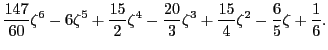
Hint: Use the command compan.
Plot these roots as points in the complex plane and draw a unit circle for comparison. (Hint: hold, real, imag).
Solution:
  bdf6 = [147/60 -6 15/2 -20/3 15/4 -6/5 1/6];
  R = eig(compan(bdf6));
  plot(R,'+'); hold on
  plot(exp(pi*i*[0:.01:2]));
  if any(find(abs(R)>1))
    fprintf('BDF6 is unstable\n');
  else
    fprintf('BDF6 is stable\n');
  end
![\includegraphics[height=8cm]{bdf6}](http://math.jacobs-university.de/oliver/teaching/iub/resources/octave/octave-intro/img44.png)
5.4 3D plot
Plot the graph of the function
Solution:
  x = -3:0.1:3;
  [xx,yy] = meshgrid(x,x);
  z = exp(-xx.^2-yy.^2);
  figure, mesh(x,x,z);
  title('exp(-x^2-y^2)');
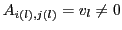
5.5 Hilbert matrix
For each ![]() Hilbert matrix
Hilbert matrix ![]() where
where ![]() compute the solution to the linear system
compute the solution to the linear system ![]() ,
, ![]() ones(n,1). Calculate the error and the condition number of the matrix and plot both in semi-logarithmic coordinates. (Hint: hilb, invhilb.)
ones(n,1). Calculate the error and the condition number of the matrix and plot both in semi-logarithmic coordinates. (Hint: hilb, invhilb.)
Solution:
  err = zeros(15,1); co = zeros(15,1);
  for k = 1:15
    H = hilb(k);
    b = ones(k,1);
    err(k) = norm(H\b-invhilb(k)*b);
    co(k) = cond(H);
  end
  semilogy(1:15,err,'r',1:15,co,'x');
5.6 Least square fit of a straight line
Calculate the least square fit of a straight line to the points ![]() , given as two vectors
, given as two vectors ![]() and
and ![]() . Plot the points and the line.
. Plot the points and the line.
Solution:
  function coeff = least_square (x,y)
    n = length(x);
    A = [x ones(n,1)];
    coeff = A\y;
    plot(x,y,'x');
    hold on
    interv = [min(x) max(x)];
    plot(interv,coeff(1)*interv+coeff(2));
  end
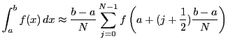
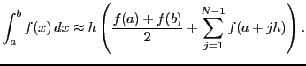
5.7 Trapezoidal rule
Write a program to integrate an arbitrary function ![]() in one variable on an interval
in one variable on an interval ![]() numerically using the trapezoidal rule with
numerically using the trapezoidal rule with ![]() :
:
For a function ![]() of your choice, check, by generating a doubly logarithmic error plot, that the trapezoidal rule is of order
of your choice, check, by generating a doubly logarithmic error plot, that the trapezoidal rule is of order ![]() .
.
Solution:
  function S = trapez(fun,a,b,N)
    h = (b-a)/N;
    % fy = feval(fun,[a:h:b]); better:
    fy = feval(fun,linspace(a,b,N+1));
    fy(1) = fy(1)/2;
    fy(N+1) = fy(N+1)/2;
    S = h*sum(fy);
  end

  function y = f(x)
    y = exp(x);
  end

  for k=1:15;
    err(k) = abs(exp(1)-1-trapez('f',0,1,2^k));
  end
  loglog(1./2.^[1:15],err);
  hold on;
  title('Trapezoidal rule, f(x) = exp(x)');
  xlabel('Increment');
  ylabel('Error');
  loglog(1./2.^[1:15],err,'x');
No hay comentarios:
Publicar un comentario